Event-study regression with a pre-trend test

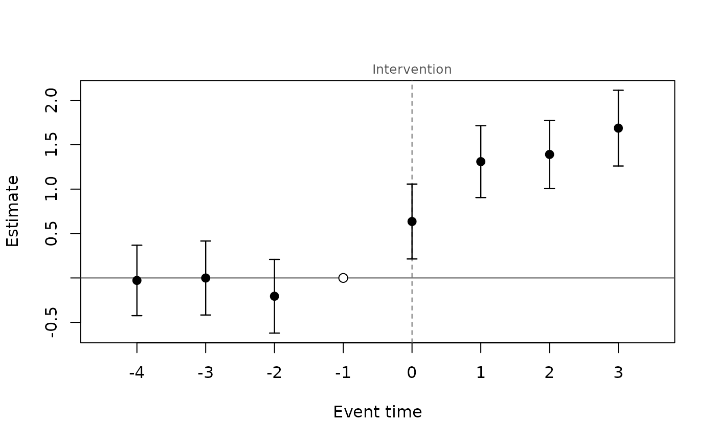
Replaces the single treatment indicator of did() by indicators of event time e = t - first treated period, from -leads to lags, with e = ref (by default the period before treatment) as the omitted reference, in a two-way fixed-effects model. Event times beyond the window are binned into the end points (bin = TRUE) or dropped from the sample (bin = FALSE). The lead coefficients estimate differences in trends before treatment; their joint Wald test is the usual check of parallel pre-trends (Freyaldenhoven et al. 2019). The lag coefficients trace the effect over time since treatment.

Usage

eventstudy(
  formula,
  data,
  index,
  treat,
  leads = 4,
  lags = 4,
  ref = -1,
  bin = TRUE,
  family = "gaussian",
  vcov = "cluster",
  level = 0.95,
  ...
)

Arguments

formula

outcome and control variables, e.g. y ~ age or y ~ 1; the treatment indicator is added

data

a data.frame in long format

index

c(individual, time); the time index must be numeric

treat

name of the column holding each individual's first treated period (in the units of the time index); NA, 0 or Inf for units that are never treated

leads, lags

number of pre- and post-treatment event times in the window (event times -leads, ..., lags)

ref

omitted reference event time, default -1

bin

logical; bin event times outside the window into the end points (TRUE) or drop those observations (FALSE)

family

"gaussian", "poisson", "negbin" or "binomial" (conditional logit, logit link only; see Details)

vcov

covariance type, cluster-robust by individual by default

level

confidence level of the reported intervals

...

further arguments passed to panglm()

Value

an object of class "panglm_eventstudy": a list with fit (the panglm() fit), estimates (a data frame with event, estimate, se, lower, upper; the reference row is zero) and pretrend (the joint test of the leads, from jointtest()) and call (the eventstudy() call, also stored as the call of fit). Methods: print, summary, coef, vcov, confint, logLik, nobs, plot, tidy and glance.

Details

Identification of all event-time coefficients needs never-treated units or a window narrower than the observed event times; without them a second coefficient is dropped (with a warning). With staggered adoption and heterogeneous effects the TWFE event-study coefficients are contaminated by effects from other periods (Sun and Abraham 2021); use a heterogeneity-robust estimator such as attgt() or etwfe() there.

With family = "binomial" the model is the two-way conditional logit (see did()) and the event-time coefficients are log odds ratios relative to the reference event time.

Validation

Numerical accuracy is checked in the package tests and in the validation suite; see the validation article on the package website.

References

Freyaldenhoven, S., Hansen, C. and Shapiro, J. M. (2019). Pre-event trends in the panel event-study design. American Economic Review, 109, 3307-3338. doi:10.1257/aer.20180609

Sun, L. and Abraham, S. (2021). Estimating dynamic treatment effects in event studies with heterogeneous treatment effects. Journal of Econometrics, 225, 175-199. doi:10.1016/j.jeconom.2020.09.006

See also

eventstudy-methods and plot.panglm_eventstudy() for the fitted model, tidy-methods for tidy() and glance().

Other policy evaluation: attgt(), did(), etwfe(), eventplot(), panelplot(), treatmentplot(), trendplot()

Examples

set.seed(1)
d <- expand.grid(id = 1:200, year = 2015:2022)
d$first <- ifelse(d$id <= 100, 2019, NA)
a <- rnorm(200)
e <- d$year - d$first
d$visits <- 3 + a[d$id] + 0.1 * (d$year - 2015) +
  ifelse(!is.na(e) & e >= 0, 0.5 + 0.4 * e, 0) + rnorm(nrow(d))
es <- eventstudy(visits ~ 1, data = d, index = c("id", "year"),
                 treat = "first", leads = 4, lags = 3)
es
#> 
#> Event study (two-way fixed effects, gaussian)
#> n = 1600  groups = 200  vcov: cluster 
#> Reference event time: -1 (end points binned) 
#> 
#>  event   estimate     se   lower  upper
#>     -4 -0.0279406 0.2023 -0.4245 0.3686
#>     -3 -0.0006271 0.2125 -0.4170 0.4158
#>     -2 -0.2058470 0.2117 -0.6209 0.2092
#>     -1  0.0000000 0.0000  0.0000 0.0000
#>      0  0.6355992 0.2152  0.2139 1.0573
#>      1  1.3096956 0.2064  0.9051 1.7143
#>      2  1.3908680 0.1949  1.0089 1.7728
#>      3  1.6868941 0.2176  1.2604 2.1134
#> 
#> Pre-trend test: Chi-squared = 1.248, df = 3, p-value = 0.7414
plot(es)