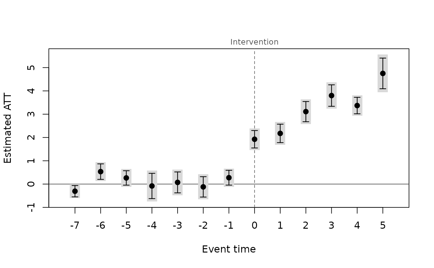
Group-time average treatment effects for staggered adoption

The Callaway and Sant'Anna (2021) estimator of the group-time average treatment effects on the treated ATT(g, t): the effect at period t for the cohort of individuals first treated at period g. Each ATT(g, t) is a two-group, two-period comparison of the change in the outcome between a base period and period t for cohort g against a clean control group (never-treated individuals, or individuals not yet treated by period t), so that already-treated individuals are never used as controls. This avoids the negative weights of the two-way fixed-effects regression of did() under staggered adoption with heterogeneous effects. The ATT(g, t) are then aggregated into an overall effect, an event study (effect by time since treatment), effects by cohort or by calendar period with summary.panglm_attgt().

Usage

attgt(
  formula,
  data,
  index,
  treat,
  control = c("never", "notyet"),
  method = c("dr", "ipw", "reg"),
  base = c("varying", "universal"),
  anticipation = 0,
  level = 0.95,
  weights = NULL,
  cluster = NULL,
  bstrap = FALSE,
  cband = FALSE,
  biters = 1000,
  multiplier = c("rademacher", "mammen"),
  seed = NULL
)

Arguments

formula: outcome ~ 1, or outcome ~ covariates for conditional parallel trends (covariates are taken in the base period)
data: a data.frame in long format
index: c(individual, time); the time index must be numeric
treat: name of the column holding each individual's first treated period (in the units of the time index); NA, 0 or Inf for units that are never treated
control: comparison group: "never" (never-treated individuals) or "notyet" (never treated or not yet treated, nor anticipating treatment, at both periods compared)
method: "dr" (doubly robust), "ipw" or "reg"; only matters with covariates
base: base period for pre-treatment ATT(g, t): "varying" or "universal"
anticipation: number of periods before g in which treatment can already affect the outcome (the base period moves back accordingly)
level: confidence level of the reported intervals
weights: optional sampling weights: the name of a column of data or a numeric vector with one value per row of data. They must be non-negative and constant within each individual (rows with a missing weight are dropped). The weights enter the propensity score, the outcome regression and the means of every ATT(g, t), and the cohort shares used by the aggregations, as weightsname in did::att_gt().
cluster: optional name of a column of data (or a vector with one value per row) defining clusters of individuals, constant within each individual (for example the region of a province). Standard errors, the pre-trend test and the bootstrap are then clustered at that level instead of the individual level.
bstrap: logical: multiplier bootstrap standard errors (FALSE by default: analytic standard errors)
cband: logical: uniform confidence bands from the bootstrap simultaneous critical value (implies bstrap = TRUE)
biters: number of bootstrap draws
multiplier: bootstrap multipliers: "rademacher" (-1 or 1 with equal probabilities, as in current versions of did) or "mammen" (the two-point distribution of Mammen 1993)
seed: optional integer seed for the bootstrap draws. When given, the draws are reproducible and the global random number generator is left as it was; otherwise a seed is drawn from it. Either way the seed is stored in the fit and reused by summary.panglm_attgt().

Value

an object of class "panglm_attgt": a list with estimates (a data frame with group, time, event (time - group), estimate, se, lower, upper and post), inf (the matrix of influence functions, one row per individual and one column per ATT(g, t)), units (individual identifiers, cohorts, normalized weights and clusters), pretrend (the Wald test of the pre-treatment ATT(g, t), or NULL), n (individuals), groups, periods, boot (with the bootstrap: the settings, the analytic standard errors se_analytic and the simultaneous critical value crit; NULL otherwise) and the settings. With cband = TRUE, estimates also has the uniform band band_lower, band_upper. Methods: print, summary, coef, vcov, nobs, plot, tidy and glance.

Estimators

With y ~ 1 (no covariates) every ATT(g, t) is the difference between the mean outcome change of cohort g and that of the control group, whatever method. With covariates, parallel trends is assumed to hold conditionally on them; their values in the base period (the earlier of the two periods compared) are used, and the comparison is made by

method = "dr": the doubly robust estimator of Sant'Anna and Zhao (2020): a logit propensity score for belonging to cohort g and a linear regression of the outcome change among controls; consistent if either model is correct;
method = "ipw": normalized inverse probability weighting with the logit propensity score;
method = "reg": outcome regression (the linear regression of the outcome change fitted on the controls, averaged over the treated).

Controls with a propensity score of 0.995 or more are trimmed, as in the DRDID package. The panel is balanced first (individuals not observed in every period are dropped), individuals already treated in the first period are dropped, and cohorts first treated after the last period are treated as never treated. When no individual is never treated, the last cohort to be treated serves as the never-treated group and the periods from its treatment date onwards are dropped (the convention of did::att_gt()).

With base = "varying" (the default) pre-treatment ATT(g, t) compare period t with period t - 1, which gives placebo estimates of the change in trends; with base = "universal" every ATT(g, t) is measured against the last period before treatment, g - 1 - anticipation, whose own ATT is zero. Post-treatment effects are the same either way.

Inference

Standard errors are analytic and come from the influence function of each estimator, including the estimation of the propensity score and outcome regression and, for the aggregations, of the cohort shares used as weights; they are robust to serial correlation within individuals. They match did::att_gt(bstrap = FALSE) and did::aggte(). With cluster, the influence functions are summed within clusters (which must nest individuals) before computing the standard errors, as clustervars in did. The joint Wald test of all pre-treatment ATT(g, t) is reported as a test of parallel pre-trends.

With bstrap = TRUE, the standard errors come instead from the multiplier bootstrap of did: each bootstrap draw multiplies the (cluster sums of the) influence functions by independent Rademacher or Mammen weights, and the standard error is the interquartile range of the draws divided by that of the standard normal, which is robust to a few extreme draws. With cband = TRUE the bootstrap also gives the simultaneous critical value, the level quantile of the largest studentized deviation across all ATT(g, t) (or all levels of an aggregation), and the uniform confidence bands band_lower, band_upper cover all effects jointly with probability level. The aggregations of summary.panglm_attgt() reuse the same multiplier draws (they are generated from seed), so that they are coherent with the ATT(g, t). Pointwise intervals (lower, upper) use the normal critical value with the bootstrap standard errors.

Validation

Numerical accuracy is checked in the package tests and in the validation suite; see the validation article on the package website.

References

Callaway, B. and Sant'Anna, P. H. C. (2021). Difference-in-differences with multiple time periods. Journal of Econometrics, 225, 200-230. doi:10.1016/j.jeconom.2020.12.001

Sant'Anna, P. H. C. and Zhao, J. (2020). Doubly robust difference-in-differences estimators. Journal of Econometrics, 219, 101-122. doi:10.1016/j.jeconom.2020.06.003

Mammen, E. (1993). Bootstrap and wild bootstrap for high dimensional linear models. The Annals of Statistics, 21, 255-285. doi:10.1214/aos/1176349025

Examples

# A health insurance scheme (for example the AMO extension in Morocco)
# is rolled out region by region: provinces of region A join in 2016,
# region B in 2018, region C in 2020, and region D not before 2022.
# Outcome: outpatient visits per 1,000 inhabitants.
set.seed(1)
d <- expand.grid(province = 1:120, year = 2012:2021)
region <- rep(c(2016, 2018, 2020, NA), each = 30)
d$adoption <- region[d$province]
d$urban <- rep(runif(120), 10)[d$province]
a <- rnorm(120)
e <- d$year - d$adoption
d$visits <- 50 + 5 * a[d$province] + 0.5 * (d$year - 2012) * (1 + d$urban) +
  ifelse(!is.na(e) & e >= 0, 2 + 0.5 * e, 0) + rnorm(nrow(d))
fit <- attgt(visits ~ 1, data = d, index = c("province", "year"),
             treat = "adoption")
fit
#> 
#> Group-time average treatment effects (Callaway and Sant'Anna 2021)
#> Control group: never treated  Estimator: unconditional  Base period: varying 
#> Individuals: 120  Periods: 10  Cohorts: 2016, 2018, 2020 
#> 
#>  group time event estimate     se   lower  upper
#>   2016 2013    -3  0.04980 0.3667 -0.6689 0.7685
#>   2016 2014    -2 -0.20624 0.3555 -0.9030 0.4905
#>   2016 2015    -1  0.51057 0.3562 -0.1876 1.2087
#>   2016 2016     0  1.46657 0.3465  0.7874 2.1458
#>   2016 2017     1  1.91160 0.3555  1.2148 2.6084
#>   2016 2018     2  3.06639 0.3778  2.3260 3.8068
#>   2016 2019     3  3.65595 0.3545  2.9611 4.3508
#>   2016 2020     4  3.37037 0.3969  2.5924 4.1484
#>   2016 2021     5  4.74969 0.3996  3.9665 5.5329
#>   2018 2013    -5  0.13987 0.3942 -0.6327 0.9124
#>   2018 2014    -4  0.33442 0.3838 -0.4178 1.0866
#>   2018 2015    -3  0.40285 0.3571 -0.2971 1.1028
#>   2018 2016    -2 -0.56983 0.3979 -1.3497 0.2100
#>   2018 2017    -1  0.07017 0.3971 -0.7080 0.8484
#>   2018 2018     0  2.47584 0.3390  1.8113 3.1403
#>   2018 2019     1  2.64339 0.4468  1.7676 3.5192
#>   2018 2020     2  3.15397 0.4152  2.3402 3.9678
#>   2018 2021     3  3.94272 0.4166  3.1263 4.7592
#>   2020 2013    -7 -0.30628 0.3614 -1.0147 0.4021
#>   2020 2014    -6  0.53454 0.3951 -0.2398 1.3089
#>   2020 2015    -5  0.38756 0.3811 -0.3593 1.1344
#>   2020 2016    -4 -0.49767 0.3251 -1.1349 0.1396
#>   2020 2017    -3 -0.23621 0.3614 -0.9445 0.4720
#>   2020 2018    -2  0.41508 0.4280 -0.4237 1.2539
#>   2020 2019    -1  0.24006 0.3168 -0.3809 0.8610
#>   2020 2020     0  1.82935 0.3836  1.0776 2.5811
#>   2020 2021     1  1.97049 0.2993  1.3839 2.5570
#> 
#> Pre-trend test: Chi-squared = 17.36, df = 15, p-value = 0.2978
#> summary(x, type = ...) gives the simple, dynamic, group or calendar
#> aggregation.
#> 
summary(fit)                     # overall ATT
#> 
#> Callaway and Sant'Anna group-time ATT
#> Aggregation: overall (simple weighted average)
#> Control group: never treated  Estimator: unconditional  Individuals: 120 
#> 
#> ATT: 2.853 (SE 0.2018, 95% CI 2.458 to 3.248)
#> 
#> Pre-trend test (pre-treatment ATT(g, t) = 0): Chi-squared = 17.36, df = 15, p-value = 0.2978
#> 
summary(fit, type = "dynamic")   # event study
#> 
#> Callaway and Sant'Anna group-time ATT
#> Aggregation: event study (by time since treatment)
#> Control group: never treated  Estimator: unconditional  Individuals: 120 
#> 
#> ATT (mean of e >= 0): 3.188 (SE 0.2282, 95% CI 2.741 to 3.635)
#> 
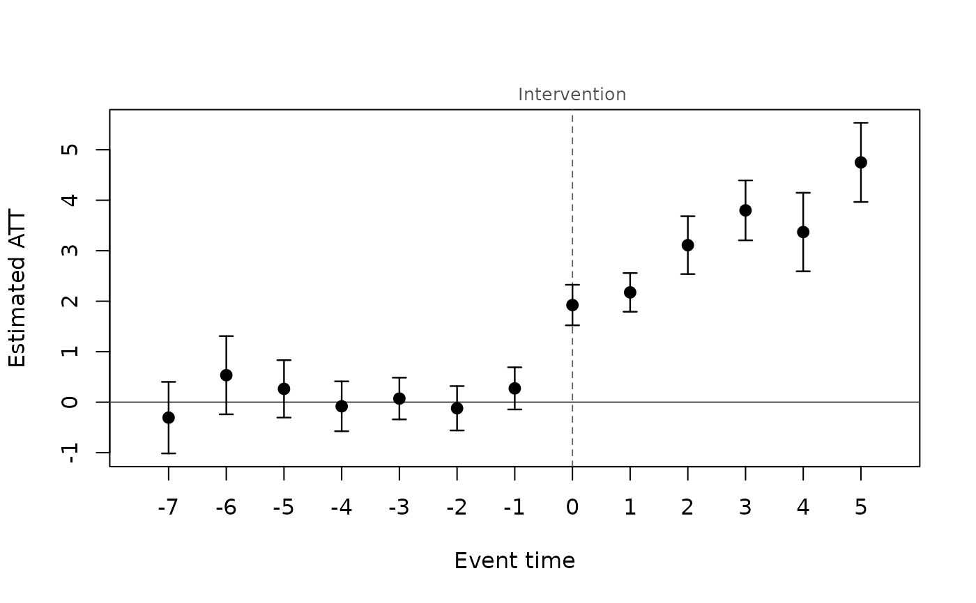
#>  event estimate     se   lower  upper
#>     -7 -0.30628 0.3614 -1.0147 0.4021
#>     -6  0.53454 0.3951 -0.2398 1.3089
#>     -5  0.26372 0.2901 -0.3049 0.8323
#>     -4 -0.08162 0.2521 -0.5756 0.4124
#>     -3  0.07214 0.2109 -0.3412 0.4855
#>     -2 -0.12033 0.2242 -0.5597 0.3190
#>     -1  0.27360 0.2129 -0.1437 0.6909
#>      0  1.92392 0.2049  1.5223 2.3256
#>      1  2.17516 0.1956  1.7918 2.5585
#>      2  3.11018 0.2923  2.5373 3.6830
#>      3  3.79934 0.3027  3.2060 4.3927
#>      4  3.37037 0.3969  2.5924 4.1484
#>      5  4.74969 0.3996  3.9665 5.5329
#> 
#> Pre-trend test (pre-treatment ATT(g, t) = 0): Chi-squared = 17.36, df = 15, p-value = 0.2978
#> 
summary(fit, type = "group")
#> 
#> Callaway and Sant'Anna group-time ATT
#> Aggregation: by treatment cohort
#> Control group: never treated  Estimator: unconditional  Individuals: 120 
#> 
#> ATT (cohort-size weighted): 2.664 (SE 0.1918, 95% CI 2.288 to 3.039)
#> 
#>  group estimate     se lower upper
#>   2016    3.037 0.2875 2.473 3.600
#>   2018    3.054 0.3343 2.399 3.709
#>   2020    1.900 0.2999 1.312 2.488
#> 
#> Pre-trend test (pre-treatment ATT(g, t) = 0): Chi-squared = 17.36, df = 15, p-value = 0.2978
#> 
plot(fit)

# conditional parallel trends (trends differ by urbanization)
fitx <- attgt(visits ~ urban, data = d, index = c("province", "year"),
              treat = "adoption", control = "notyet", method = "dr")
summary(fitx, type = "dynamic")
#> 
#> Callaway and Sant'Anna group-time ATT
#> Aggregation: event study (by time since treatment)
#> Control group: not yet treated  Estimator: DR  Individuals: 120 
#> 
#> ATT (mean of e >= 0): 3.226 (SE 0.1746, 95% CI 2.884 to 3.569)
#> 
#>  event  estimate     se   lower  upper
#>     -7 -0.369291 0.2944 -0.9463 0.2077
#>     -6  0.492471 0.3390 -0.1719 1.1569
#>     -5  0.153830 0.2463 -0.3290 0.6366
#>     -4  0.006396 0.2183 -0.4214 0.4342
#>     -3 -0.020909 0.1885 -0.3903 0.3485
#>     -2 -0.129620 0.2215 -0.5638 0.3046
#>     -1  0.224753 0.1905 -0.1487 0.5982
#>      0  1.974815 0.1797  1.6226 2.3270
#>      1  2.206638 0.1933  1.8278 2.5855
#>      2  3.196001 0.2521  2.7020 3.6900
#>      3  3.826915 0.2391  3.3583 4.2955
#>      4  3.382490 0.3564  2.6839 4.0811
#>      5  4.770903 0.3268  4.1303 5.4115
#> 
#> Pre-trend test (pre-treatment ATT(g, t) = 0): Chi-squared = 18.1, df = 15, p-value = 0.2575
#> 
# multiplier bootstrap, clustered by region, with uniform bands
d$region <- ceiling(d$province / 10)
fitb <- attgt(visits ~ 1, data = d, index = c("province", "year"),
              treat = "adoption", cluster = "region", cband = TRUE,
              biters = 499, seed = 1)
#> Warning: the simultaneous critical value is very large (7.62) and may be unreliable
plot(fitb)