Fit a generalized linear model for panel data

Fast pooled, fixed-effects ("within") and random-effects panel GLMs, backed by an Rcpp/RcppArmadillo/RcppParallel numerical core. See the package vignette for the estimators currently implemented per family.

Usage

panglm(
  formula,
  data,
  index,
  model = c("pooling", "within", "random", "between"),
  family = "gaussian",
  weights = NULL,
  offset = NULL,
  na.action = stats::na.omit,
  effect = c("individual", "twoways"),
  vcov = c("classical", "HC1", "cluster"),
  cre = dynamic,
  dynamic = FALSE,
  random = ~1,
  R = 21,
  maxit = 100,
  tol = 1e-10
)

Arguments

formula: a model formula, e.g. y ~ x1 + x2. lag(x, k), lead(x, k) and diff(x) are taken within each individual on the grid of sorted distinct time values (see "Lags and differences" in panglm(); needs index = c(id, time)); the first waves of each individual get NA and leave the sample, and lag(x, 0:2) gives several lags
data: a data.frame containing the variables in formula and index
index: length-1 or length-2 character vector identifying the individual (and optionally time) columns, e.g. c("id", "time")
model: one of "pooling", "within", "random", "between". The between estimator (family = "gaussian" only) is least squares on the individual means of the outcome and the regressors, one row per individual, as in plm(model = "between"); it uses only the variation between individuals and is the cross-sectional counterpart of the within estimator. Its robust covariances ("HC1", "cluster") are the same, since each individual is one observation of the means regression.
family: one of "gaussian", "poisson", "binomial", "probit", "negbin", "gamma", "ologit", "oprobit", "beta", "tobit", or a family spec from gaussianfamily() / poissonfamily() / binomialfamily() / negbinfamily() / gammafamily() / orderedfamily() / betafamily() / tobitfamily(). Base R family objects with a matching distribution and link are also accepted and mapped onto these: stats::gaussian(), stats::poisson(), stats::binomial("logit"), stats::binomial("probit") and stats::Gamma("log"); other stats families stop with an error naming the panglm constructor to use.
weights: optional nonnegative observation (prior) weights: the name of a column of data or a numeric vector with one value per row of data, e.g. inverse probability weights for attrition. Nontrivial weights are supported for model = "pooling" (all families); the fit then maximizes the weighted (pseudo) log-likelihood and robust covariances use the weighted scores. For model = "random" the weights must be constant within individuals (one weight per individual, e.g. a baseline sampling weight) and the fit maximizes the weighted sum of the individual integrated log-likelihoods; the Gaussian model is then estimated by maximum likelihood instead of Swamy-Arora FGLS. Use vcov = "cluster" for design-based standard errors. Weighted fixed-effects fits are rejected.
offset: optional model offset (the name of a column of data or a numeric vector with one value per row of data). Nonzero offsets, including offsets specified in formula, are rejected explicitly rather than ignored.
na.action: missing-data action passed to stats::model.frame()
effect: one of "individual" or "twoways" (individual + time fixed effects). "twoways" is implemented for model = "within" only: family = "gaussian" (iterative alternating-projections demeaning, iterated until it converges to tolerance, with a warning if the limit of 10,000 sweeps is reached first), "poisson" and "negbin" (both via outer-IRLS / inner-weighted-FWL, the algorithm behind fixest::feglm()), and "binomial", the two-way conditional (Chamberlain) logit: the individual effects are conditioned out exactly and the time effects are estimated as time dummies inside the conditional likelihood, as in survival::clogit(y ~ x + factor(time) + strata(id), method = "exact"). For the two-way logit coef() holds the slopes only; the time effects (first time level as reference, NA when not identified) and their standard errors are in fit$time_effects and fit$time_effects_se, and the classical and robust covariances of the slopes account for their estimation.
vcov: one of "classical", "HC1" (heteroskedasticity-robust) or "cluster" (cluster-robust, clustered by the panel individual by default). For model = "random" only "classical" and "cluster" are available; the cluster covariance uses the individual scores of the integrated likelihood, so clusters must contain whole individuals. See vcov.panglm() to recompute a different type after fitting.
cre: logical. If TRUE, fit a correlated random effects (Mundlak) model: the individual means of every time-varying regressor are added to the design matrix, named mean_<column>. Available for model = "pooling" and model = "random" and every family. The slopes of the time-varying regressors then have a within interpretation, and the joint Wald test of the mean terms is a Hausman-type (Mundlak) test, reported by summary.panglm() with the covariance stored on the fit: it is robust to heteroskedasticity and within-individual correlation only when that covariance is (vcov = "cluster", or "HC1" for heteroskedasticity alone); with the default classical covariance it assumes the model's error structure. Defaults to dynamic.
dynamic: logical. If TRUE, fit a dynamic model with the Wooldridge (2005) solution to the initial conditions problem: the outcome of the previous wave (lag_<y>) and the outcome of the first observed wave (initial_<y>) are added to the regressors, the first wave is dropped, and the individual means of the time-varying regressors are added (cre = TRUE by default; the lag is not averaged). The second element of index must be a numeric time variable; a lag is only defined when the previous wave t - 1 is observed, other rows are dropped. Factor and logical outcomes (ordered and binary models) give factor or logical lags, so their partial effects are discrete changes. With model = "random" the coefficient of the lag measures true state dependence net of unobserved heterogeneity; partialeffects() gives it on the probability or mean scale. Available for model = "pooling" and model = "random".
random: one-sided formula for the random effects of model = "random". The default ~ 1 is the random intercept. A formula with variables, e.g. ~ time, adds correlated random slopes: g(E[y_it | b_i]) = x_it' beta + z_it' b_i with z_it = (1, time) and b_i ~ N(0, Sigma), Sigma unstructured (Cholesky parameterized), the model of lme4::lmer(y ~ x + (1 + time | id)). The slope variables usually also appear in formula (their average slope). Available for family = "gaussian" (exact maximum likelihood, any number of slopes), and for "poisson", "negbin" (NB2, the model of glmmTMB::nbinom2(), with theta stored as negbin_theta), "gamma" (log link, the model of glmmTMB with Gamma(link = "log"), shape stored as shape) and "binomial" (logit or probit), with any number of slopes, by adaptive Gauss-Hermite product quadrature with R nodes per dimension, R^q nodes for q random effects; R = 1 is the Laplace approximation of lme4::glmer() and glmmTMB. With random slopes the random effects are always normal on the link scale, so for "poisson" and "negbin" the multiplicative effect exp(z_it' b_i) is lognormal. These are different models from the random-intercept fits of random = ~ 1: the random-intercept "poisson" model uses gamma mixing (the conjugate model of Hausman, Hall and Griliches, whose likelihood is in closed form, as Stata's xtpoisson, re) and the random-intercept "negbin" model is the beta-mixed negative binomial of Hausman, Hall and Griliches (Stata's xtnbreg, re), whereas with random slopes "negbin" is NB2 with a lognormal effect, as glmmTMB::nbinom2(). Adding a slope whose variance is estimated at zero therefore does not reproduce the random = ~ 1 fit for these two families: the slope coefficients keep their conditional (rate ratio) meaning, but the intercept (E[exp(b_i)] = exp(sigma^2 / 2) under lognormal mixing against 1 under gamma mixing), the variance parameters and the log-likelihood differ. For "binomial" and "gamma" the random-intercept models are already normal on the link scale and are the zero-slope special case. The fit stores varcomp (the covariance matrix Sigma), ranef (posterior modes, the BLUPs in the Gaussian model, one row per individual) and, for the Gaussian model, the residual variance sigma_v2. Weights, dynamic = TRUE and the other families are not supported with random slopes; cre = TRUE is. Response predictions and partialeffects() are population averages over the random effects.
R: number of adaptive Gauss-Hermite quadrature nodes for the random-effects models whose likelihood has no closed form: binomial (logit, probit), gamma, ordered, beta and Tobit. The default R = 21 reproduces lme4::glmer(nAGQ = 21) and ordinal::clmm(nAGQ = 21) to about 1e-5 in the coefficients and the log-likelihood (for a probit model with a large random-intercept spread, say sigma > 1.5, raise R to 41 or more for that accuracy). The nodes are centred at the mode of each individual's integrand and scaled by its curvature, so R = 1 is the Laplace approximation (with the observed curvature, except for the beta model, which uses the expected one). R is ignored by the closed-form random-intercept Gaussian, Poisson and negative binomial models. With random slopes, R is the number of nodes per dimension of the adaptive product rule; when it is not given it is 7 for one slope, 5 for two, 3 for three to five and 1 (Laplace) beyond, so that R^q stays moderate, and a warning is given when R^q exceeds 2000.
maxit: maximum IRLS/Newton iterations
tol: convergence tolerance

Value

an object of class "panglm" (with the additional class "panordered" for the ordered families): a list with coefficients, vcov, vcov_type, fitted.values, linear.predictors, loglik, the variance components of random-effects fits (sigma_mu2, sigma_v2, theta), the panel structure, nobs, n_groups, call and formula. Methods: print, summary, coef, vcov, confint, predict, fitted, residuals, logLik, nobs, model.matrix, plot, partialeffects(), effectcurve(), tidy and glance.

Lags and differences

Inside the formula, lag(x, k), lead(x, k) and diff(x, lag, differences) are taken within each individual, never across individuals. Shifts step through the sorted distinct values of the time index, so lag(x, 1) is the value at the previous observed wave. With gaps in the time index this differs from plm: for waves coded 2010, 2012, 2014, lag(x, 1) at 2012 is the 2010 value in panglm, while plm::lag() (which shifts by the numeric time value) gives NA. To obtain plm's behaviour, keep a row for every period, with NA outcomes for the missing waves. pangmm() uses the same rule. The first k waves of each individual get NA and leave the estimation sample. diff() follows base R's diff(x, lag, differences); plm's third argument of diff() is shift, not differences. The same rule applies in paniv(), panqr() and panfmm().

Validation

Numerical accuracy is checked in the package tests and in the validation suite; see the validation article on the package website.

Examples

data(copd)

# pooled OLS on lung function (ignores the panel structure)
fit_pool <- panglm(fev1 ~ treatment + age + smoker + crp, data = copd,
                    index = c("id", "visit"), model = "pooling", family = "gaussian")
summary(fit_pool)
#> 
#> Call:
#> panglm(formula = fev1 ~ treatment + age + smoker + crp, data = copd, 
#>     index = c("id", "visit"), model = "pooling", family = "gaussian")
#> 
#> Family: gaussian  Link: identity  Model: pooling  Effect: individual 
#> n = 300  groups = 60  vcov: classical 
#> 
#> Coefficients:
#>              Estimate Std. Error z value Pr(>|z|)    
#> (Intercept)  4.091479   0.225597  18.136  < 2e-16 ***
#> treatment    0.208556   0.056578   3.686 0.000228 ***
#> age         -0.014239   0.003133  -4.545  5.5e-06 ***
#> smoker      -0.355207   0.055905  -6.354  2.1e-10 ***
#> crp         -0.032895   0.013135  -2.504 0.012269 *  
#> ---
#> Signif. codes:  0 ‘***’ 0.001 ‘**’ 0.01 ‘*’ 0.05 ‘.’ 0.1 ‘ ’ 1
#> 
#> Log-likelihood: -189.6 
#> Dispersion parameter: 0.2107 
#> Residual df: 295  Iterations: 2
#> 

# fixed-effects ("within") estimator: only the time-varying regressor
# (crp) survives demeaning; time-invariant covariates like treatment
# or age are not identified by a fixed-effects estimator
fit_fe <- panglm(fev1 ~ crp, data = copd,
                  index = c("id", "visit"), model = "within", family = "gaussian")
coef(fit_fe)
#>         crp 
#> -0.03530482 

# random-effects (Swamy-Arora) estimator
fit_re <- panglm(fev1 ~ treatment + age + smoker + crp, data = copd,
                  index = c("id", "visit"), model = "random", family = "gaussian")
coef(fit_re)
#> (Intercept)   treatment         age      smoker         crp 
#>  4.10943890  0.20549733 -0.01430869 -0.35583462 -0.03519775 

# fixed-effects Poisson on exacerbation counts
fit_pois <- panglm(exacerbations ~ crp, data = copd,
                    index = c("id", "visit"), model = "within", family = "poisson")
coef(fit_pois)
#>        crp 
#> 0.05112674 

# correlated random effects (Mundlak) probit for hospitalization
fit_cre <- panglm(hospitalized ~ treatment + age + crp, data = copd,
                  index = c("id", "visit"), model = "random",
                  family = "probit", cre = TRUE)
summary(fit_cre)
#> 
#> Call:
#> panglm(formula = hospitalized ~ treatment + age + crp, data = copd, 
#>     index = c("id", "visit"), model = "random", family = "probit", 
#>     cre = TRUE)
#> 
#> Family: binomial  Link: probit  Model: random  Effect: individual 
#> n = 300  groups = 60  vcov: classical 
#> 
#> Coefficients:
#>             Estimate Std. Error z value Pr(>|z|)    
#> (Intercept) -2.72956    1.07767  -2.533 0.011315 *  
#> treatment   -0.47330    0.22839  -2.072 0.038231 *  
#> age          0.03989    0.01126   3.544 0.000394 ***
#> crp          0.05887    0.04543   1.296 0.194948    
#> mean_crp    -0.12856    0.11532  -1.115 0.264932    
#> ---
#> Signif. codes:  0 ‘***’ 0.001 ‘**’ 0.01 ‘*’ 0.05 ‘.’ 0.1 ‘ ’ 1
#> 
#> Log-likelihood: -159.8 
#> Dispersion parameter: 1 
#> Random-intercept SD: 0.2689 
#> Mundlak test (individual means jointly zero): chi2(1) = 1.243, p = 0.2649
#> Residual df: 294  Iterations: 31
#> 

# patient trajectories: random intercept and random slope of FEV1
# decline per visit, correlated
fit_rs <- panglm(fev1 ~ visit + treatment + age + smoker, data = copd,
                 index = c("id", "visit"), model = "random",
                 random = ~ visit)
#> Warning: the random-effects covariance matrix is singular (on the boundary of the parameter space): the variance of 'visit' given the preceding random effects is estimated at zero; consider a simpler 'random' formula
summary(fit_rs)
#> 
#> Call:
#> panglm(formula = fev1 ~ visit + treatment + age + smoker, data = copd, 
#>     index = c("id", "visit"), model = "random", random = ~visit)
#> 
#> Family: gaussian  Link: identity  Model: random  Effect: individual 
#> n = 300  groups = 60  vcov: classical 
#> 
#> Coefficients:
#>              Estimate Std. Error z value Pr(>|z|)    
#> (Intercept)  3.872439   0.414554   9.341  < 2e-16 ***
#> visit       -0.004717   0.008262  -0.571  0.56808    
#> treatment    0.251411   0.110762   2.270  0.02322 *  
#> age         -0.013627   0.006396  -2.131  0.03312 *  
#> smoker      -0.342166   0.114817  -2.980  0.00288 ** 
#> ---
#> Signif. codes:  0 ‘***’ 0.001 ‘**’ 0.01 ‘*’ 0.05 ‘.’ 0.1 ‘ ’ 1
#> 
#> Log-likelihood: -38.65 
#> Dispersion parameter: 0.04087 
#> Random effects (SD): (Intercept) 0.42204, visit 0.00297 
#> Random-effects correlation: visit ~ (Intercept) -1 
#> Residual df: 295  Iterations: 18
#> 
fit_rs$varcomp
#>              (Intercept)         visit
#> (Intercept)  0.178115898 -1.253281e-03
#> visit       -0.001253281  8.818484e-06

# two-way conditional logit: smoking across survey waves, with year
# shocks (e.g. a tobacco tax) absorbed by the time effects
set.seed(1)
smk <- expand.grid(wave = 1:5, id = 1:200)
smk$price <- rnorm(nrow(smk)) + 0.2 * smk$wave
smk$smoking <- rbinom(nrow(smk), 1, plogis(rnorm(200)[smk$id] - 0.5 * smk$price +
                                               c(0, 0.2, -0.3, -0.6, -0.8)[smk$wave]))
fit_2w <- panglm(smoking ~ price, data = smk, index = c("id", "wave"),
                 model = "within", family = "binomial", effect = "twoways",
                 vcov = "cluster")
#> 37 group(s) with no within-group outcome variation dropped (all-0 or all-1) -- they carry no information for the conditional likelihood.
summary(fit_2w)
#> 
#> Call:
#> panglm(formula = smoking ~ price, data = smk, index = c("id", 
#>     "wave"), model = "within", family = "binomial", effect = "twoways", 
#>     vcov = "cluster")
#> 
#> Family: binomial  Link: logit  Model: within  Effect: twoways 
#> n = 1000  groups = 200  vcov: cluster 
#> 
#> Coefficients:
#>       Estimate Std. Error z value Pr(>|z|)    
#> price -0.57501    0.08186  -7.024 2.15e-12 ***
#> ---
#> Signif. codes:  0 ‘***’ 0.001 ‘**’ 0.01 ‘*’ 0.05 ‘.’ 0.1 ‘ ’ 1
#> 
#> Log-likelihood: -282.3 
#> Dispersion parameter: 1 
#> Iterations: 5
#> 
fit_2w$time_effects
#>          1          2          3          4          5 
#>  0.0000000  0.3259111 -0.2093176 -0.4856443 -0.5288287 

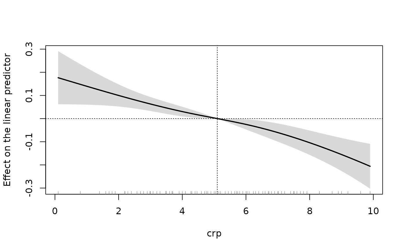
# nonlinear effect through a natural spline: linearity test and curve
fit_ns <- panglm(fev1 ~ splines::ns(crp, 3), data = copd,
                 index = c("id", "visit"), model = "within", vcov = "cluster")
lineartest(fit_ns, "crp")
#> 
#> Joint Wald test (vcov: cluster)
#> H0: the effect of crp is linear 
#> Chi-squared = 1.338, df = 2, p-value = 0.5122
#> 
plot(effectcurve(fit_ns, "crp"))