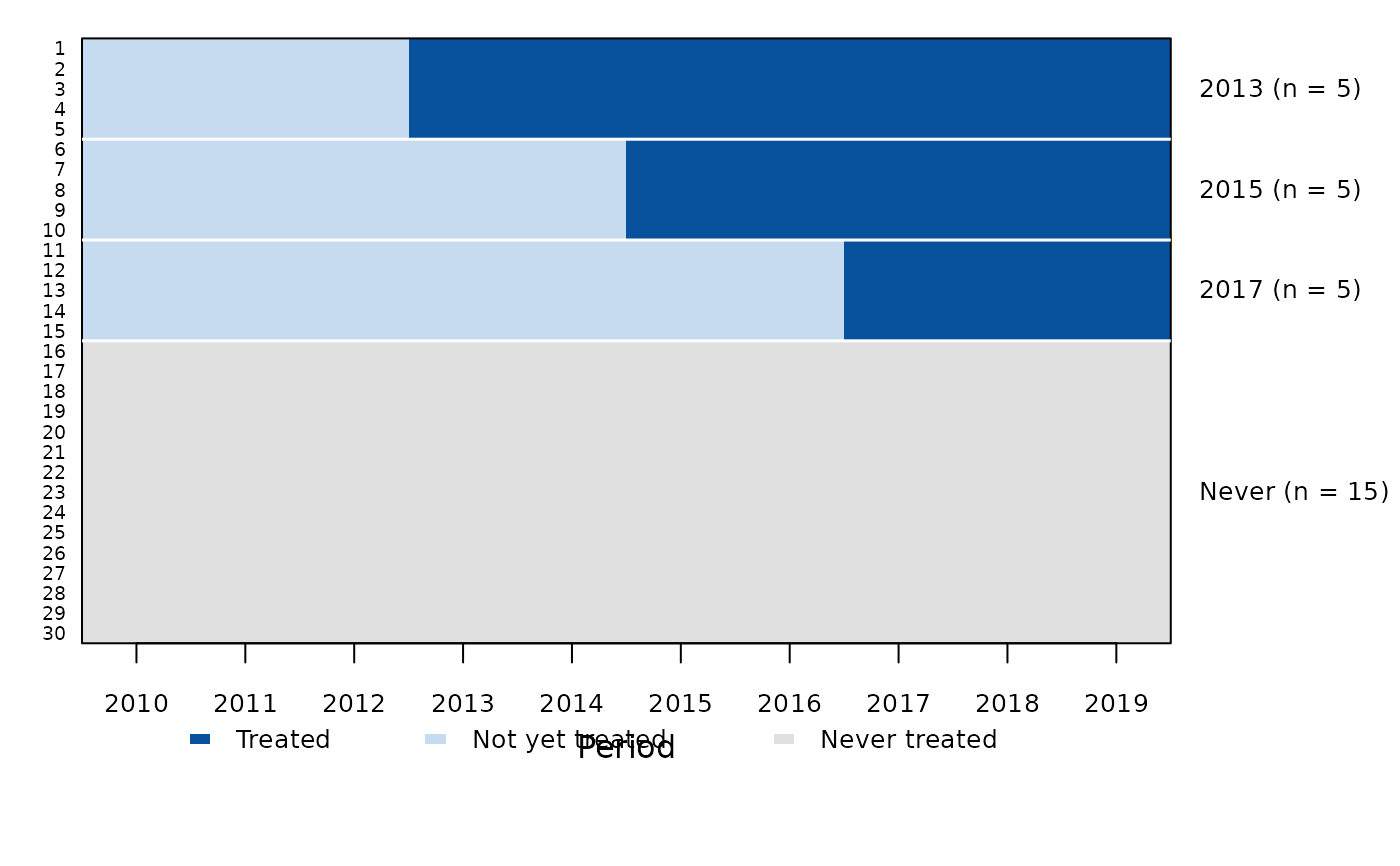
Draws one row per individual and one column per period, sorted by treatment cohort (earliest adopters at the top, never-treated units at the bottom), with treated cells shaded. The right axis gives each cohort and its size. With many individuals the unit labels are dropped and the tiles are drawn as a raster, so the plot stays readable for thousands of units. Periods in which a unit is not observed are left blank.
Usage
treatmentplot(
  data,
  index,
  treat,
  labels = NULL,
  col = c("#08519C", "#C6DBEF", "grey88"),
  legend = TRUE,
  xlab = "Period",
  ylab = NULL,
  main = NULL,
  ...
)
Arguments
- data
a data frame in long format
- index
c(individual, time): column names, the time numeric- treat
name of the column with the first treated period, as in
attgt()andetwfe()(0,NAorInffor never-treated units)- labels
logical: show the individual labels on the left axis. The default shows them for at most 60 individuals.
- col
colours of the treated, not-yet-treated and never-treated cells
- legend
logical: add a legend below the plot
- xlab, ylab, main
axis labels and title
- ...
passed to
graphics::image()
See also
Other policy evaluation:
attgt(),
did(),
etwfe(),
eventplot(),
eventstudy(),
panelplot(),
trendplot()
Examples
d <- expand.grid(id = 1:30, year = 2010:2019)
d$first <- rep(c(2013, 2015, 2017, 0, 0, 0), each = 5)[d$id]
treatmentplot(d, index = c("id", "year"), treat = "first")