Extended two-way fixed-effects difference-in-differences

The extended two-way fixed-effects (ETWFE) estimator of Wooldridge (2021, 2023) for staggered adoption, with linear, Poisson or logit outcome models. The model interacts the treatment with every cohort by period cell, so that each cohort can have its own effect in each period: with g the first treated period of the cohort and t the period, $$E[y_{it}] = F(\alpha + \gamma_g + \lambda_t + \sum_{(g, t)} \tau_{gt} D_{gt,it} + x_{it}'\beta + \ldots)$$ where D_gt indicates cohort g in period t, gamma_g and lambda_t are cohort and period effects and F is the identity, the exponential or the logistic function. Because the cell effects are unrestricted, the estimator does not suffer from the negative weights of the single-coefficient TWFE regression of did(); in the linear case with control = "notyet" it is numerically equivalent to an imputation estimator. For nonlinear models, parallel trends is imposed on the index (for example on the log of the mean for Poisson), which suits counts and binary outcomes.

Usage

etwfe(
  formula,
  data,
  index,
  treat,
  family = c("gaussian", "poisson", "binomial", "logit"),
  control = c("notyet", "never"),
  vcov = c("cluster", "classical"),
  level = 0.95,
  weights = NULL,
  xvar = NULL,
  ivar = FALSE
)

Arguments

formula: outcome ~ 1, or outcome ~ controls
data: a data.frame in long format
index: c(individual, time); the time index must be numeric. The individual identifies the clusters for the standard errors.
treat: name of the column holding each individual's first treated period; NA, 0 or Inf for units that are never treated
family: "gaussian" (linear), "poisson" (counts, log link) or "binomial" (binary, logit link; "logit" is accepted)
control: "notyet" or "never"; see Specification
vcov: "cluster" (by individual, the default) or "classical". The cluster covariance uses the factor G / (G - 1) * (n - 1) / (n - k) with k counting all coefficients, cohort and period dummies included (with ivar = TRUE, the individual effects, nested in the clusters, count as one), as fixest does.
level: confidence level of the reported intervals
weights: optional sampling weights: the name of a column of data or a non-negative numeric vector with one value per row (rows with a missing weight are dropped). They weight the quasi-likelihood (as weights = ~w in etwfe::etwfe() and fixest) and the averages of the treatment effects over the treated observations in summary.panglm_etwfe() (as wts in etwfe::emfx()). The centring of the controls at their cohort means (and of xvar at its cell means) is unweighted, as in etwfe. Unlike in attgt(), the weights need not be constant within individuals: the model is a weighted pooled (quasi-)likelihood over the rows, so observation-level weights are well defined, and the cluster-robust covariance by individual remains valid (as in fixest). Use weights constant within individuals when they are sampling weights of the individuals, so that the estimates are comparable with attgt().
xvar: optional name of one numeric or logical column of data: a covariate by which the treatment effects may vary (see Heterogeneity by a covariate)
ivar: logical; TRUE uses individual (the first element of index) instead of cohort fixed effects, for family = "gaussian" only (see Specification)

Value

an object of class "panglm_etwfe": a list with coefficients, vcov, cells (a data frame of the cohort by period cells with their coefficient on the index scale), family, control, reference (the reference cohort), xvar, ivar, nobs, n_groups, the design (X, y, rows) and the call. Methods: print, summary (the ATTs), coef, vcov, nobs, plot, tidy and glance.

Details

The average treatment effects on the treated are then computed on the response scale as marginal effects: for each treated observation, the difference between the predicted mean with its cell effect and without it, averaged over the treated observations (all of them, by cohort, by calendar period or by time since treatment; see summary.panglm_etwfe()). Standard errors use the delta method with analytic gradients.

Specification

Cohort and period effects enter as dummies (cohort effects rather than individual effects: for linear models on balanced panels without time-varying controls the two give the same cell effects, and for nonlinear models the pooled quasi-likelihood with cohort dummies is the estimator of Wooldridge 2023). With control = "notyet" (the default) the cell dummies cover the post-treatment cells only, so all untreated observations, of never-treated and not-yet-treated cohorts, identify the counterfactual. With control = "never" every cell of each treated cohort gets a dummy except the period just before treatment, so only never-treated individuals identify the period effects and the pre-treatment cells give placebo estimates. The reference cohort is the never-treated group; without never-treated individuals and with control = "notyet" the last cohort to be treated is the reference and the periods from its treatment date onwards are dropped. Individuals treated in the first period are dropped.

Control variables in formula enter with their main effect, their interactions with the cohort and period dummies, and interactions of the cell dummies with the control variables centred at their cohort means, as in Wooldridge (2021) and the etwfe package, so that the cell effects can vary with the controls.

With ivar = TRUE (linear model only) individual fixed effects replace the cohort effects, as ivar in etwfe::etwfe(): they are swept out by within-individual demeaning (weighted when there are weights). On a balanced panel without time-varying controls the cell effects and ATTs are the same as with cohort effects. They differ with time-varying controls (the individual effects then also absorb the part of the individual heterogeneity that is correlated with the controls, as the Mundlak means of Wooldridge 2021 would) and on unbalanced panels; the individual effects also absorb time-invariant controls. Nonlinear models keep the cohort effects (with few periods, individual effects in a logit model suffer from the incidental parameters problem; the pooled Poisson and logit quasi-likelihoods with cohort effects are the estimators of Wooldridge 2023), and ivar = TRUE is an error there, whereas etwfe::etwfe() ignores ivar for nonlinear families.

Heterogeneity by a covariate

xvar names a covariate by which the treatment effects may vary, as xvar in etwfe::etwfe() (typically a time-invariant indicator, such as sex, rural residence or a baseline risk group). The covariate is centred at its cohort by period cell means and enters through its interactions with the period dummies (except the first period) and with every cell dummy, so each cohort by period effect becomes a linear function of the covariate, with the cell coefficient as the effect at the cell mean. This is the specification of the etwfe package; the level of the covariate itself is not a regressor, so add it to formula as a control to adjust for it as well. summary.panglm_etwfe() then reports the ATTs separately for each value of the covariate (byxvar = TRUE, the default for such a fit), as etwfe::emfx(by_xvar = TRUE); with a continuous covariate there is one row per distinct value, so summarise a binary or discrete version of it.

Validation

Numerical accuracy is checked in the package tests and in the validation suite; see the validation article on the package website.

References

Wooldridge, J. M. (2021). Two-way fixed effects, the two-way Mundlak regression, and difference-in-differences estimators. Working paper. doi:10.2139/ssrn.3906345

Wooldridge, J. M. (2023). Simple approaches to nonlinear difference-in-differences with panel data. The Econometrics Journal, 26, C31-C66. doi:10.1093/ectj/utad016

Examples

# Staggered rollout of a health insurance scheme by region (for example
# RAMED, then AMO, in Morocco): regions join in 2016, 2018 or 2020, the
# last region not before 2022. Outcome: number of hospital admissions
# per district and year (a count).
set.seed(1)
d <- expand.grid(district = 1:160, year = 2012:2021)
d$adoption <- rep(c(2016, 2018, 2020, NA), each = 40)[d$district]
d$poverty <- rep(runif(160), 10)[d$district]
a <- rnorm(160, sd = 0.3)
treated <- !is.na(d$adoption) & d$year >= d$adoption
d$admissions <- rpois(nrow(d), exp(2 + a[d$district] + 0.03 * (d$year - 2012) +
                                    0.2 * treated))
fit <- etwfe(admissions ~ 1, data = d, index = c("district", "year"),
             treat = "adoption", family = "poisson")
fit                                   # overall ATT, admissions per district
#> 
#> Extended TWFE (Wooldridge), Poisson model, control group: not yet treated
#> Observations: 1600  Individuals: 160  vcov: cluster 
#> Fixed effects: cohort and period
#> 
#> ATT (response scale): 1.606 (SE 0.3506, 95% CI 0.9193 to 2.294, p = 4.606e-06)
#> 
#> summary(x, type = ...) gives effects by group, calendar period or event time.
#> 
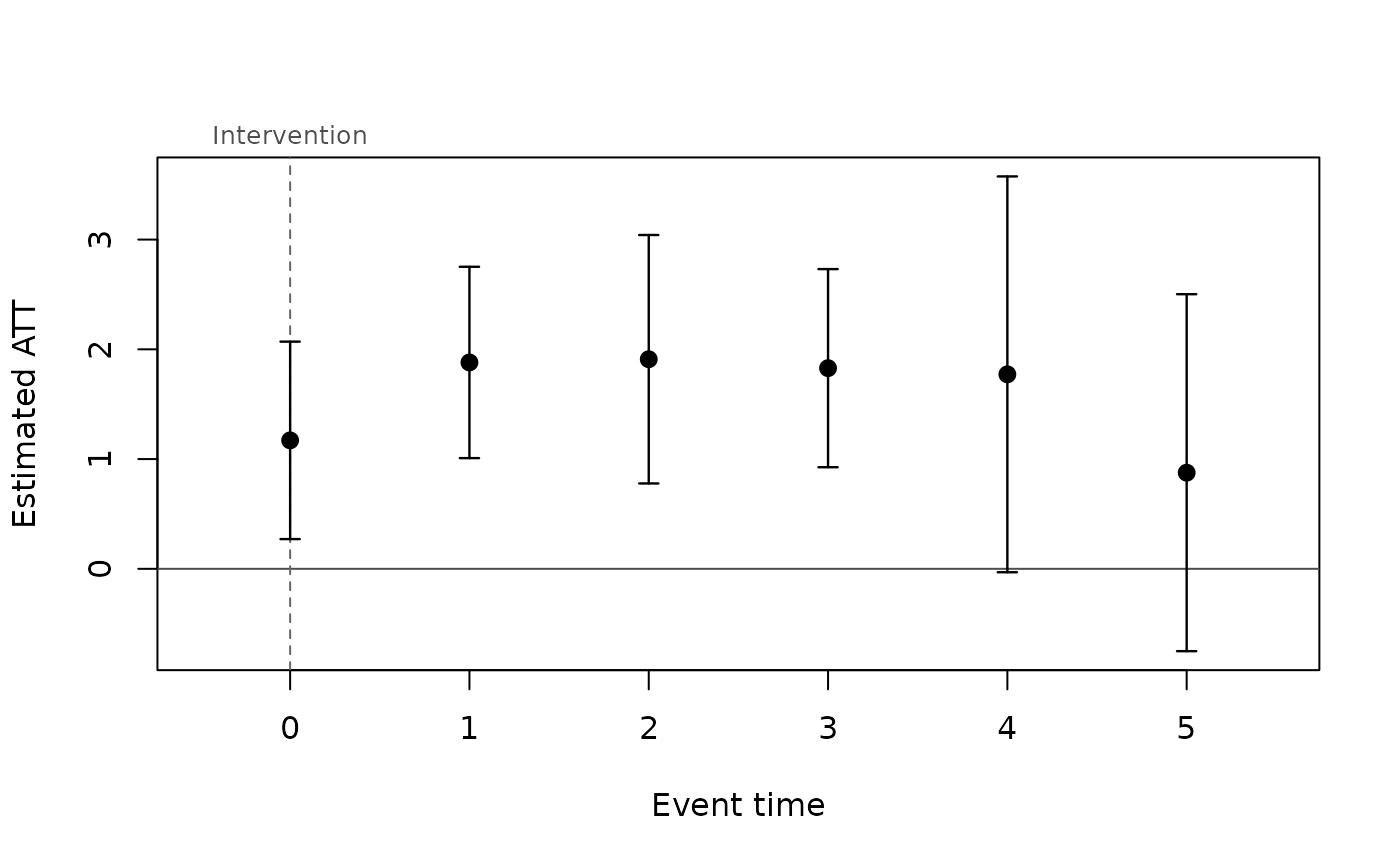
summary(fit, type = "event")          # by time since adoption
#> 
#> Extended TWFE (Wooldridge), Poisson model, control group: not yet treated
#> Observations: 1600  Individuals: 160  vcov: cluster 
#> Fixed effects: cohort and period
#> 
#> ATT (response scale): 1.606 (SE 0.3506, 95% CI 0.9193 to 2.294, p = 4.606e-06)
#> 
#>  event estimate     se statistic   p.value    lower upper
#>      0    1.171 0.4590     2.550 1.076e-02  0.27095 2.070
#>      1    1.880 0.4448     4.228 2.361e-05  1.00867 2.752
#>      2    1.910 0.5775     3.307 9.434e-04  0.77788 3.042
#>      3    1.828 0.4605     3.970 7.179e-05  0.92582 2.731
#>      4    1.772 0.9201     1.926 5.409e-02 -0.03116 3.575
#>      5    0.876 0.8298     1.056 2.911e-01 -0.75036 2.502
#> 
summary(fit, type = "group")
#> 
#> Extended TWFE (Wooldridge), Poisson model, control group: not yet treated
#> Observations: 1600  Individuals: 160  vcov: cluster 
#> Fixed effects: cohort and period
#> 
#> ATT (response scale): 1.606 (SE 0.3506, 95% CI 0.9193 to 2.294, p = 4.606e-06)
#> 
#>  group estimate     se statistic   p.value    lower upper
#>   2016    1.483 0.4206     3.525 4.229e-04  0.65845 2.307
#>   2018    1.963 0.4139     4.743 2.109e-06  1.15185 2.774
#>   2020    1.264 0.6932     1.823 6.826e-02 -0.09473 2.622
#> 
plot(fit)

# linear model with a control variable
d$visits <- 50 + 5 * a[d$district] + 0.5 * (d$year - 2012) + 2 * treated +
  rnorm(nrow(d))
summary(etwfe(visits ~ poverty, data = d, index = c("district", "year"),
              treat = "adoption"), type = "calendar")
#> 
#> Extended TWFE (Wooldridge), linear model, control group: not yet treated
#> Observations: 1600  Individuals: 160  vcov: cluster 
#> Fixed effects: cohort and period
#> 
#> ATT (response scale): 2.019 (SE 0.1086, 95% CI 1.806 to 2.232, p = < 2.2e-16)
#> 
#>  time estimate     se statistic   p.value lower upper
#>  2016    1.907 0.2257     8.450 2.901e-17 1.465 2.350
#>  2017    1.737 0.1912     9.087 1.020e-19 1.363 2.112
#>  2018    2.136 0.1593    13.413 5.043e-41 1.824 2.448
#>  2019    2.039 0.1732    11.773 5.386e-32 1.699 2.378
#>  2020    1.977 0.2078     9.516 1.795e-21 1.570 2.384
#>  2021    2.100 0.2121     9.901 4.113e-23 1.684 2.515
#> 
# individual instead of cohort fixed effects (linear model)
summary(etwfe(visits ~ poverty, data = d, index = c("district", "year"),
              treat = "adoption", ivar = TRUE), type = "group")
#> 
#> Extended TWFE (Wooldridge), linear model, control group: not yet treated
#> Observations: 1600  Individuals: 160  vcov: cluster 
#> Fixed effects: individual and period
#> 
#> ATT (response scale): 2.019 (SE 0.1083, 95% CI 1.806 to 2.231, p = < 2.2e-16)
#> 
#>  group estimate     se statistic   p.value lower upper
#>   2016    2.003 0.1310     15.30 7.935e-53 1.747 2.260
#>   2018    2.043 0.1299     15.73 8.990e-56 1.788 2.297
#>   2020    2.017 0.1942     10.39 2.884e-25 1.636 2.397
#> 
# effects by a covariate: poor versus other districts
d$poor <- as.numeric(d$poverty > 0.5)
fx <- etwfe(admissions ~ 1, data = d, index = c("district", "year"),
            treat = "adoption", family = "poisson", xvar = "poor")
summary(fx)                           # ATT for poor = 0 and poor = 1
#> 
#> Extended TWFE (Wooldridge), Poisson model, control group: not yet treated
#> Observations: 1600  Individuals: 160  vcov: cluster 
#> Fixed effects: cohort and period; effects by poor
#> 
#> ATT (response scale): 1.607 (SE 0.3525, 95% CI 0.9157 to 2.297, p = 5.172e-06)
#> 
#>  poor estimate     se statistic   p.value   lower upper
#>     0    1.042 0.5836     1.786 0.0740359 -0.1013 2.186
#>     1    2.220 0.5914     3.754 0.0001744  1.0607 3.379
#> 
summary(fx, type = "event", byxvar = FALSE)
#> 
#> Extended TWFE (Wooldridge), Poisson model, control group: not yet treated
#> Observations: 1600  Individuals: 160  vcov: cluster 
#> Fixed effects: cohort and period
#> 
#> ATT (response scale): 1.607 (SE 0.3525, 95% CI 0.9157 to 2.297, p = 5.172e-06)
#> 
#>  event estimate     se statistic   p.value   lower upper
#>      0   1.1708 0.4615     2.537 1.118e-02  0.2663 2.075
#>      1   1.8806 0.4406     4.269 1.967e-05  1.0171 2.744
#>      2   1.9098 0.5772     3.308 9.381e-04  0.7784 3.041
#>      3   1.8284 0.4671     3.914 9.075e-05  0.9128 2.744
#>      4   1.7726 0.9183     1.930 5.358e-02 -0.0273 3.572
#>      5   0.8761 0.8286     1.057 2.904e-01 -0.7479 2.500
#>