Plot raw outcome trends of a difference-in-differences design

Draws the mean outcome over time, the classical first look at a difference-in-differences design before any model is fitted.

Usage

trendplot(
  data,
  index,
  treat,
  outcome,
  type = c("cohort", "treated", "event"),
  weights = NULL,
  band = FALSE,
  level = 0.95,
  min_e = -Inf,
  max_e = Inf,
  col = NULL,
  legend = TRUE,
  xlab = NULL,
  ylab = NULL,
  main = NULL,
  ylim = NULL,
  ...
)

Arguments

data: a data frame in long format
index: c(individual, time): column names, the time numeric
treat: name of the column with the first treated period, as in attgt() and treatmentplot() (0, NA or Inf for never-treated units)
outcome: name of the outcome column (numeric or logical)
type: "cohort", "treated" or "event" (see Details)
weights: optional sampling weights: the name of a column of data or a non-negative numeric vector with one value per row
band: logical: add pointwise confidence bands (shaded) around each line
level: confidence level of the bands
min_e, max_e: event window for type = "event"
col: line colours, one per line (cohorts first, the never treated last). The default gives ordered colours to the cohorts and black to the never treated.
legend: logical: add a legend
xlab, ylab, main: axis labels and title
ylim: y-axis limits
...: passed to graphics::plot()

Value

a data frame of the plotted means, invisibly: group (the line label), time (calendar period, or event time for type = "event"), mean, se and n (number of observations)

Details

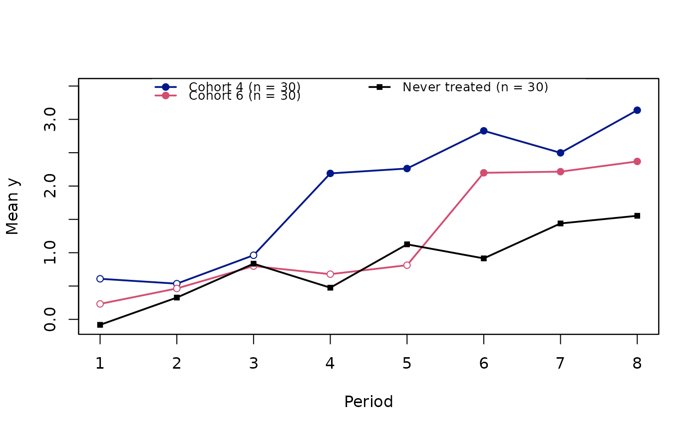
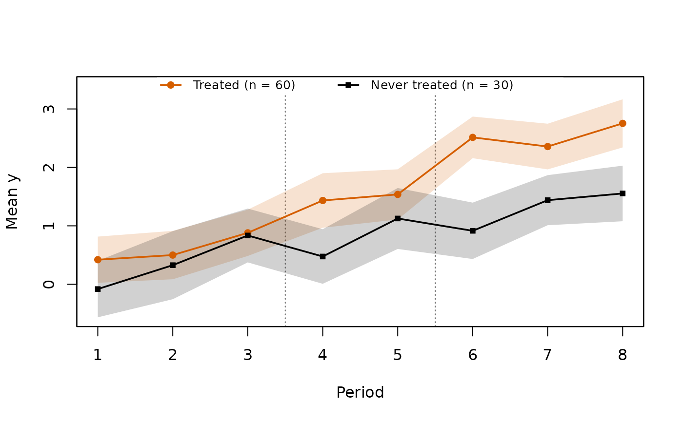
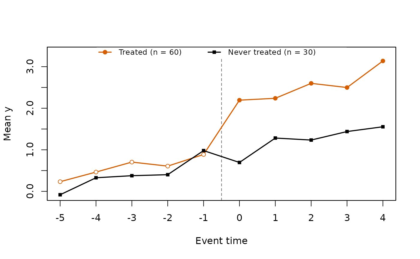
type = "cohort": one line per adoption cohort and one for the never-treated units, against calendar time. Points are hollow before the cohort adopts and filled from adoption on.
type = "treated": the ever-treated and never-treated means against calendar time. A dashed vertical line marks a single adoption date (half a period before it); with staggered adoption each adoption date gets a dotted line (the ever-treated mean then mixes treated and not yet treated observations).
type = "event": the treated units aligned on event time (period minus first treated period), with a dashed line at treatment onset (-0.5). Never-treated units have no event time, so their mean cannot be aligned directly; the never-treated line is instead their mean in the same calendar periods as the treated observations: at event time e, each treated observation contributes the never-treated mean of its own period (a calendar-matched comparison, as in stacked event studies). The treated mean at each event time pools cohorts observed in different calendar periods, so its composition changes with e.

Means are weighted by weights when given. The standard error of each mean is cluster-robust by individual, $$\widehat{se}(\bar y_c) = \sqrt{\frac{G_c}{G_c - 1} \sum_{g} \Big(\sum_{i \in g} w_i (y_i - \bar y_c)\Big)^2 \Big/ W_c^2},$$ with G_c the number of individuals contributing to the mean and W_c the sum of their weights: the usual standard error of a mean (with one observation per individual it is s / sqrt(n)), and the one of fixest::feols(y ~ 1, cluster = ~id) fitted on the observations of the mean. The calendar-matched never-treated line of type = "event" is a fixed linear combination of period means; its standard error uses the same formula with the influence of each never-treated observation.

Examples

set.seed(2)
d <- expand.grid(id = 1:90, t = 1:8)
d$first <- rep(c(4, 6, 0), each = 30)[d$id]
d$y <- rnorm(90)[d$id] + 0.2 * d$t +
  ifelse(d$first > 0 & d$t >= d$first, 1, 0) + rnorm(nrow(d))
trendplot(d, index = c("id", "t"), treat = "first", outcome = "y")

trendplot(d, c("id", "t"), "first", "y", type = "treated", band = TRUE)

m <- trendplot(d, c("id", "t"), "first", "y", type = "event")

head(m)
#>     group time      mean        se  n
#> 1 Treated   -5 0.2322927 0.3041021 30
#> 2 Treated   -4 0.4638733 0.2999028 30
#> 3 Treated   -3 0.7041348 0.1874108 60
#> 4 Treated   -2 0.6071081 0.2158302 60
#> 5 Treated   -1 0.8873404 0.2011706 60
#> 6 Treated    0 2.1941933 0.1964449 60