Technical reference: models, estimators and inference

This vignette is the technical reference of panglm. It states the models, the estimating equations and the covariance estimators, and defines the scope of the package. Worked examples are in the task vignettes:

Topic	Vignette
Data layout, pooled, within, between, random and correlated random effects, standard errors, partial effects, tables	vignette("panglm-intro")
Counts, hurdle, two-part costs, beta, ordered and tobit models	vignette("panglm-outcomes")
Instrumental variables, Hausman-Taylor, dynamic GMM, sample selection	vignette("panglm-endogeneity")
Difference-in-differences, event studies, staggered adoption	vignette("panglm-policy")
Random slopes, latent classes, quantile regression	vignette("panglm-heterogeneity")

The numerical routines use Rcpp, RcppArmadillo and RcppParallel.

library(panglm)
data(copd)

Notation and data organization

Let $y_{it}$ be the response of unit $i = 1, \dots, N$ at occasion $t = 1, \dots, T_i$, and $x_{it}$ a vector of covariates. The conditional mean is linked to a linear predictor by

$$g\{E(y_{it} \mid x_{it}, \alpha_i, \gamma_t)\} = x_{it}^{\mathsf T}\beta + \alpha_i + \gamma_t,$$

where $\alpha_i$ is an individual effect and $\gamma_t$ an optional time effect. index names the individual and time variables. model sets how $\alpha_i$ is treated:

• "pooling" omits $\alpha_i$;
• "within" treats $\alpha_i$ as a fixed nuisance parameter;
• "between" regresses individual means on individual means;
• "random" gives $\alpha_i$ a distribution and integrates it out.

effect = "twoways" adds the time effects to supported fixed-effects models.

Model matrices follow the usual R formula rules. Before estimation the rank is checked after the transformation of the requested estimator; unidentified columns, such as time-invariant regressors in a within model, are reported and dropped. Missing responses or covariates follow na.action; missing or duplicated index pairs are errors. Nonzero offsets are rejected. Observation weights are accepted by pooled models and, when constant within individuals, by random-effects models.

Linear estimators

Pooled. Least squares, or iteratively reweighted least squares (IRLS) for generalized linear models. The negative binomial model uses the NB2 variance $\mu_{it} + \mu_{it}^2/\theta$ and alternates coefficient updates with the estimation of $\theta$. With prior weights $w_{it}$ the score is $\sum_{it} w_{it} s_{it}(\beta)$; zero weights remove an observation from the fit, the likelihood and the degrees of freedom. Robust and cluster covariances use the weighted scores and treat the weights as known, which is the usual inverse probability weighting for attrition.

Within. The one-way estimator is least squares on $\tilde y_{it} = y_{it} - \bar y_i$ and $\tilde x_{it} = x_{it} - \bar x_i$. With effect = "twoways" alternating projections remove both individual and time means; they are iterated until the largest change in a sweep is below tolerance (one sweep for a balanced panel), which also handles unbalanced panels, and a warning is given if the iteration limit is reached first.

Between. Least squares on the individual means, $\bar y_i = \bar x_i^{\mathsf T}\beta + \bar u_i$, one row per individual. Its HC1 covariance equals the cluster covariance because each individual contributes one row.

Random effects. The Gaussian model is the Swamy and Arora (1972) feasible GLS estimator: with $\lambda_i = 1 - \sigma_\varepsilon / (\sigma_\varepsilon^2 + T_i\sigma_\alpha^2)^{1/2}$ it regresses $y_{it} - \lambda_i \bar y_i$ on $x_{it} - \lambda_i \bar x_i$, with variance components from the within and between residuals. In a balanced panel $\hat\sigma_\alpha^2 = s_b^2 - \hat\sigma_\varepsilon^2 / T$ with $s_b^2$ the residual variance of the between regression. In an unbalanced panel the between regression weights each individual by $T_i$ and the variance components solve the trace-based moment equations of plm (random.method = "swar"), which reduce to the balanced ones when all $T_i$ are equal. A negative $\hat\sigma_\alpha^2$ is set to zero with a warning. With weights, or with random slopes, the Gaussian model is fitted by maximum likelihood instead.

Nonlinear fixed effects

Poisson. For one-way models the individual intercept has the closed-form profile solution $\hat\alpha_i(\beta) = \log\{Y_i / L_i(\beta)\}$, with $Y_i = \sum_t y_{it}$ and $L_i(\beta) = \sum_t \exp(x_{it}^{\mathsf T}\beta)$. Substitution gives the conditional Poisson estimator (Hausman, Hall and Griliches 1984), which is consistent for fixed $T$ when the conditional mean is correct. Two-way models use an outer IRLS loop with weighted alternating projections (Guimaraes and Portugal 2010).

Negative binomial. The one-way NB2 model estimates the slopes, one intercept per individual and $\theta$ jointly (Allison and Waterman 2002); all-zero groups are dropped with a message. It is not the conditional negative binomial model of Hausman, Hall and Griliches (1984), whose scale restriction does not remove an individual intercept. Dummy intercepts do not remove the finite-$T$ incidental parameter bias in general, so short panels call for caution.

Gamma. With $E(y_{it} \mid x_{it}, \alpha_i) = \exp(\alpha_i + x_{it}^{\mathsf T}\beta)$ the gamma log-link estimator with one intercept per individual is consistent for fixed $T$ under strict exogeneity, because its concentrated score has mean zero, as for the Poisson model. The log-link working weights are constant, so each IRLS step is a within regression.

Binomial. The one-way model is the exact conditional logit (Chamberlain 1980). Given $S_i = \sum_t y_{it}$, unit $i$ contributes

$$L_i(\beta \mid S_i) = \frac{\exp\left(\sum_t y_{it}x_{it}^{\mathsf T}\beta\right)} {\sum_{a:\,\sum_t a_t=S_i} \exp\left(\sum_t a_tx_{it}^{\mathsf T}\beta\right)},$$

evaluated with its score by a forward and backward recursion. Units with all-zero or all-one responses carry no information and are dropped. The likelihood is maximized by Newton-Raphson; the gradient and Hessian are exact, from the derivatives of the same recursion (the algorithm of survival::clogit(method = "exact")), and the inverse of that Hessian is the classical covariance. With effect = "twoways" the individual effects are conditioned out and time effects enter as dummies.

Ordered logit. model = "within" fits the blow-up and cluster estimator of Baetschmann, Staub and Winkelmann (2015): each observation is copied once per cutoff, dichotomized at that cutoff, and a conditional logit is fitted to the stacked data with standard errors clustered by individual.

Random-intercept likelihoods

Random-effects models integrate over $\alpha_i$:

Family	Mixing distribution	Integration
Gaussian	normal	closed form (FGLS or ML)
Poisson	gamma	closed form (negative binomial marginal)
Negative binomial	beta on the NB2 probability	closed form (Hausman, Hall and Griliches 1984)
Binomial (logit, probit)	normal on the link scale	adaptive Gauss-Hermite quadrature
Gamma, ordered, beta, tobit	normal on the link scale	adaptive Gauss-Hermite quadrature

R sets the number of quadrature nodes (default 21). Adaptive quadrature centres the nodes at each individual’s mode and scales them by the curvature there, so R = 1 is the Laplace approximation (the beta model scales by the expected curvature). For the binomial and ordered models the gradient is exact, including the dependence of the mode and the curvature on the parameters, and the default R = 21 reproduces lme4::glmer(nAGQ = 21) and ordinal::clmm(nAGQ = 21) to about 1e-5. A probit model with a large random-intercept spread needs more nodes for that accuracy: on pglm::UnionWage ($\sigma_\alpha = 1.7$) 21 nodes leave an error of about 1e-3 in the log-likelihood, and 41 or more remove it. R is ignored by the closed-form Gaussian, Poisson and negative binomial random-intercept models. Response predictions are marginal over $\alpha_i$; for the gamma model this includes the lognormal factor $\exp(\sigma_\alpha^2/2)$. Covariances use the observed information, and vcov = "cluster" gives the sandwich built from the individual scores of the integrated likelihood. With weights constant within individuals the weighted sum of the individual log-likelihoods is maximized and the cluster covariance is design based.

Correlated random effects. cre = TRUE adds the individual means of the time-varying regressors, $\alpha_i = \bar x_i^{\mathsf T}\gamma + a_i$ (Mundlak 1978; Chamberlain 1980), as mean_<variable> columns. In linear models the coefficients on $x_{it}$ then equal the within estimates. The summary reports the Wald test of $\gamma = 0$, the regression form of the Hausman test.

Dynamic models. dynamic = TRUE applies the initial-conditions solution of Wooldridge (2005): it adds the lagged outcome lag_<y>, the first observed outcome initial_<y> and the individual means of the time-varying regressors, and drops the first wave. The coefficient on lag_<y> measures state dependence.

Random slopes

random = ~ z gives the model $g\{E(y_{it} \mid b_i)\} = x_{it}^{\mathsf T}\beta + z_{it}^{\mathsf T}b_i$, with $z_{it}$ the intercept and the listed variables and $b_i \sim N(0, \Sigma)$, $\Sigma$ unstructured (Laird and Ware 1982). The Gaussian model is fitted by exact maximum likelihood. Poisson, negative binomial, gamma and binomial (logit or probit) models use adaptive Gauss-Hermite quadrature on a product grid of $R^q$ nodes, with $q$ the dimension of $b_i$; the cost therefore grows quickly with $q$. $\Sigma$ is parametrized by its Cholesky factor. The fit stores $\hat\Sigma$ in varcomp and the predicted effects (posterior modes, the BLUPs in the Gaussian case) in ranef.

Outcome-specific models

Ordered. orderedfamily("logit") or orderedfamily("probit"): $P(y_{it} \le j) = F(c_j - x_{it}^{\mathsf T}\beta - \alpha_i)$, with the intercept absorbed in the cutpoints $c_j$. Pooled and random-intercept fits for both links; the fixed-effects model above for the logit link.

Beta. betafamily(): $y_{it} \sim \mathrm{Beta}(\mu_{it}\phi, (1 - \mu_{it})\phi)$ with $g(\mu_{it}) = x_{it}^{\mathsf T}\beta$, so $\mathrm{Var}(y_{it}) = \mu_{it}(1 - \mu_{it})/(1 + \phi)$ (Ferrari and Cribari-Neto 2004). The precision is fit$precision. Responses of exactly 0 or 1 must first be moved inside the interval (Smithson and Verkuilen 2006). Regressors should be on a moderate scale.

Tobit. tobitfamily(left, right): a latent $y^*_{it} = x_{it}^{\mathsf T}\beta + \alpha_i + \varepsilon_{it}$, $\varepsilon_{it} \sim N(0, \sigma_\varepsilon^2)$, is observed as $y_{it} = \min\{\max(y^*_{it}, \ell), r\}$ (Tobin 1958). Censored observations contribute $\Phi\{(\ell - \eta_{it})/\sigma_\varepsilon\}$ or $1 - \Phi\{(r - \eta_{it})/\sigma_\varepsilon\}$, the others the normal density. Pooled and random-intercept models; the random intercept SD is fit$sigma and the error SD fit$sigma_e.

Two-part. twopart() fits the model of Duan et al. (1983), $E(y_{it}) = P(y_{it} > 0)\, E(y_{it} \mid y_{it} > 0)$, with a probit or logit first part and a gamma (log link) or lognormal positive part, pooled or with random intercepts, optionally with cre = TRUE. The lognormal retransformation uses Duan’s smearing factor (default) or $\exp(\sigma^2/2)$. With correlated = TRUE and a lognormal positive part, the two random intercepts are bivariate normal with correlation $\rho$ and both parts are fitted jointly (Van Ourti 2004). The positive part integrates in closed form given $u_{1i}$, and the integral over $u_{1i}$ uses adaptive quadrature. The marginal mean is then

$$E(y_{it}) = \exp\{z_{it}^{\mathsf T}\beta + (\sigma_e^2 + \tau^2)/2\}\, E_{u_1}\{F(x_{it}^{\mathsf T}\gamma + u_1)\, e^{c u_1}\}, \quad c = \rho\sigma_2/\sigma_1,\; \tau^2 = \sigma_2^2(1 - \rho^2).$$

Hurdle. panhurdle() fits two fixed-effects parts: a conditional logit for $1(y_{it} > 0)$ and a zero-truncated Poisson or NB2 model for the positive counts, with density $f(y \mid \mu, \theta)/\{1 - f(0 \mid \mu, \theta)\}$ for $y > 0$ and one intercept per individual.

Endogenous regressors

Two-stage least squares. paniv() takes y ~ regressors | instruments, where the second part is the full instrument set. With $\tilde a$ the within, quasi-demeaned or untransformed version of a variable and $\hat X = P_{\tilde Z}\tilde X$,

$$\hat\beta_{\mathrm{2SLS}} = (\hat X^{\mathsf T}\tilde X)^{-1} \hat X^{\mathsf T}\tilde y .$$

model = "within" and "pooling" give fixed-effects and pooled 2SLS. model = "random" gives the generalized 2SLS of Balestra and Varadharajan-Krishnakumar (inst.method = "bvk") or the EC2SLS of Baltagi (1981) ("baltagi", instruments $[QZ, PZ]$), with variance components from within and between 2SLS residuals. The summary reports the first-stage partial $R^2$ and $F$ of the excluded instruments, and a Sargan test (or a cluster-robust Hansen $J$) when overidentified.

Hausman-Taylor. model = "hausmantaylor" (Hausman and Taylor 1981) splits the regressors into time-varying and time-invariant, exogenous and endogenous with respect to $\alpha_i$. The second formula part lists the exogenous ones. The within-transformed time-varying regressors and the exogenous time-varying means and time-invariant regressors are the instruments, so the exogenous time-varying regressors must be at least as many as the endogenous time-invariant ones.

Dynamic GMM. pangmm() fits $y_{it} = \rho y_{i,t-1} + x_{it}^{\mathsf T}\beta + \alpha_i + \varepsilon_{it}$. The difference estimator of Arellano and Bond (1991) uses $E(y_{is}\Delta\varepsilon_{it}) = 0$ for $s \le t - 2$; the system estimator of Blundell and Bond (1998) (transformation = "ld") adds $E(\Delta y_{i,t-1}\varepsilon_{it}) = 0$. collapse = TRUE and maxlag limit the instrument count. The two-step covariance uses the Windmeijer (2005) correction. Reported tests: Arellano-Bond AR(1) and AR(2), Sargan and Hansen.

Sample selection. panselect() implements Wooldridge (1995). A probit for selection is fitted in each period, with the individual means of the selection regressors (mundlak = TRUE). The inverse Mills ratio, interacted with period dummies (lambda = "period") or common ("common"), enters the outcome equation, estimated by fixed effects or pooled OLS. The joint test of the Mills ratio terms is the test of selection bias; it is valid with the cluster covariance under the null. Coefficient standard errors come from a cluster bootstrap over both steps (boot replicates).

Policy evaluation

Two-way fixed effects. did() fits $g\{E(y_{it})\} = \alpha_i + \lambda_t + \delta D_{it} + x_{it}^{\mathsf T}\beta$, with $D_{it} = 1(t \ge g_i)$ and $g_i$ the first treated period. Gaussian, Poisson, negative binomial and conditional logit fits are available. Poisson TWFE needs only the conditional mean to be correct (Wooldridge 2023). eventstudy() replaces $D_{it}$ with indicators of event time $e = t - g_i$ from -leads to lags, reference ref = -1, with the end points binned by default. Its Wald test of the leads is the pre-trend test. Under staggered adoption with heterogeneous effects the TWFE coefficient is a weighted average of two-by-two comparisons with possibly negative weights (Goodman-Bacon 2021; Sun and Abraham 2021).

Group-time effects. attgt() estimates, for each cohort $g$ and period $t$,

$$\mathrm{ATT}(g, t) = E(y_t - y_{b} \mid G = g) - E(y_t - y_{b} \mid C),$$

with base period $b = g - 1$ (moved back by anticipation) and comparison group $C$ never or not yet treated (Callaway and Sant’Anna 2021). Pre-treatment ATT$(g, t)$ use the previous period as base (base = "varying") or $g - 1$ (base = "universal"). With covariates the comparison is outcome regression, inverse probability weighting or the doubly robust combination (Sant’Anna and Zhao 2020). Aggregations (summary(type = "simple", "dynamic", "group", "calendar")) weight the ATT$(g, t)$ by cohort size. Standard errors come from the influence functions, or from the multiplier bootstrap (bstrap, biters), which allows a coarser cluster and uniform bands (cband).

Extended TWFE. etwfe() (Wooldridge 2021, 2023) fits one pooled regression with cohort and period effects and a treatment indicator for every treated cohort by post-period cell; covariates enter centred at their cohort means and interacted with the cells. In the linear case the cell coefficients equal the imputation estimates of ATT$(g, t)$. With family = "poisson" or "binomial" parallel trends holds on the link scale and the effects are averaged on the response scale with delta-method standard errors. xvar gives effects by a covariate; ivar = TRUE uses unit instead of cohort effects (linear only).

Finite mixtures

panfmm() assumes each individual belongs to one of $k$ latent classes for all its observations, so the likelihood contribution is

$$L_i = \sum_{c=1}^{k} \pi_c(w_i) \prod_t f_c(y_{it} \mid x_{it}; \beta_c), \qquad \pi_c(w_i) = \frac{\exp(w_i^{\mathsf T}\delta_c)}{\sum_l \exp(w_i^{\mathsf T}\delta_l)},$$

with Gaussian, Poisson, NB2 or binomial components (Deb and Trivedi 1997, 2002) and individual-level concomitant variables $w_i$ (concomitant). EM is run from nstart random starts and the best fit kept; the covariance is the inverse observed information of the full likelihood, or its cluster sandwich. panfmmselect() compares $k$ by AIC and BIC. predict(type = "posterior") returns the posterior class probabilities.

Quantile regression

panqr() assumes $Q_{y_{it}}(\tau \mid x_{it}, \alpha_i) = \alpha_i + x_{it}^{\mathsf T}\beta(\tau)$ with location-shift individual effects.

• "canay" (Canay 2011): $\hat\alpha_i$ from the within regression, then quantreg regression of $y_{it} - \hat\alpha_i$ on $x_{it}$. Consistent as $N$ and $T$ grow. Analytic or cluster bootstrap standard errors.
• "mmqr" (Machado and Santos Silva 2019): the location-scale model $y_{it} = \alpha_i + x_{it}^{\mathsf T}\beta + (\delta_i + x_{it}^{\mathsf T}\gamma)U_{it}$, estimated by two within regressions and the $\tau$-quantile $q(\tau)$ of the standardized residuals, so $\beta(\tau) = \beta + \gamma q(\tau)$. The analytic covariance is cluster-robust by individual: the influence functions of the location, scale and $q(\tau)$ steps are summed within each cluster and $V = \frac{G}{G-1}\sum_g \psi_g\psi_g^{\mathsf T}$. vcov = "iid" gives the formula of their paper, which assumes independent observations.
• "pooling": quantreg regression ignoring $\alpha_i$, with a cluster-robust covariance.

Regression splines

Any formula term works, including splines::ns(x, df), splines::bs(x, df) and poly(x, degree). Basis columns are demeaned like any regressor in fixed-effects fits, and the knots of the estimation sample are reused by predict() and model.matrix().

• lineartest(fit, "x"): the spline basis contains the linear function, $x = c + Ba$, so linearity means the spline coefficients are proportional to $a$; the test is the joint Wald test of the $q - 1$ implied restrictions, with any covariance type.
• jointtest(fit, pattern = "x"): Wald test that all columns of x are zero.
• effectcurve(fit, "x", ref): change in the linear predictor from ref to a grid of values, with delta-method pointwise limits.

set.seed(2026)
N <- 150; TT <- 5
sim <- data.frame(id = rep(seq_len(N), each = TT), year = rep(seq_len(TT), N))
alpha <- rnorm(N)
sim$bmi <- 27 + 3 * alpha[sim$id] + rnorm(N * TT, sd = 2.5)
sim$logcost <- 6 + alpha[sim$id] + 0.004 * (sim$bmi - 23)^2 +
  rnorm(N * TT, sd = 0.4)
fit_spline <- panglm(logcost ~ splines::ns(bmi, 4), data = sim,
                     index = c("id", "year"), model = "within",
                     vcov = "cluster")
lineartest(fit_spline, "bmi")
#> 
#> Joint Wald test (vcov: cluster)
#> H0: the effect of bmi is linear 
#> Chi-squared = 28.93, df = 3, p-value = 2.316e-06

plot(effectcurve(fit_spline, "bmi", ref = 25), xlab = "Body mass index",
     ylab = "Change in log spending vs BMI 25")
curve(0.004 * (x - 23)^2 - 0.004 * (25 - 23)^2, add = TRUE, lty = 2)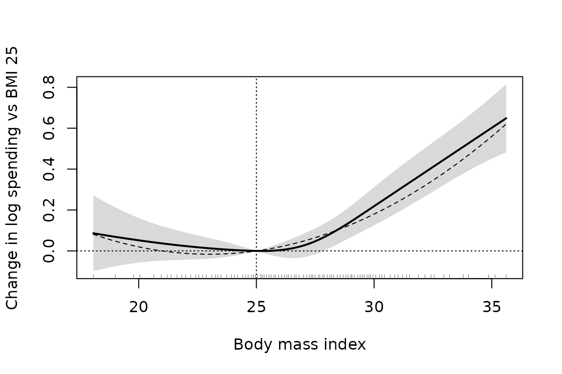

A likelihood ratio test of nested fixed-effects fits is biased upwards here: the dummy-variable error variance divides the residual sum of squares by $NT$ instead of $N(T - 1)$, which inflates the statistic by about $T/(T - 1)$. The Wald form is preferred.

Average partial effects

partialeffects() averages $\partial E(y_{it} \mid x_{it}) / \partial x_{itj}$ over the sample for continuous regressors, and the discrete change for binary and factor regressors, with delta-method standard errors from the stored covariance. For random-effects models the mean integrates over $\alpha_i$, the average structural function of Wooldridge (2005); in correlated random effects fits the individual means are held fixed. Ordered models give one effect per category; two-part models give effects on either part or on the unconditional mean.

Covariance estimation

The default covariance is model based. With $B$ the inverse information and $s_j$ the score contributions, the sandwich is

$$\hat V(\hat\beta) = B \left(\sum_j s_j(\hat\beta)s_j(\hat\beta)^{\mathsf T}\right)B .$$

"HC1" uses observation scores; "cluster" sums them within clusters first, the individual by default or a coarser cluster variable. Linear models use the finite-sample factor $G/(G - 1) \cdot (n - 1)/(n - k)$ of plm::vcovHC(type = "sss"). For the conditional logit the independent contribution is a whole stratum, so HC1 uses stratum scores and a custom cluster may combine but not split strata. For random-effects models the scores are those of the individual integrated likelihoods.

fit_fe <- panglm(fev1 ~ crp, data = copd, index = c("id", "visit"),
                 model = "within")
sqrt(c(classical = vcov(fit_fe), HC1 = vcov(fit_fe, type = "HC1"),
       cluster = vcov(fit_fe, type = "cluster")))
#>   classical         HC1     cluster 
#> 0.005974855 0.005293113 0.006071829

panhausman() compares compatible fixed- and random-effects fits with the covariance difference, or in its Mundlak form with any covariance. pandispersiontest() reports the Pearson statistic over its residual degrees of freedom for count fits.

Likelihoods and information criteria

logLik(), AIC() and BIC() count the estimated shape, dispersion, variance and absorbed fixed-effect parameters that belong to the reported likelihood. Gaussian within fits report the dummy-variable normal likelihood, and Swamy-Arora fits the exact (not REML) normal random-intercept likelihood at the FGLS estimates. Conditional Poisson and conditional logit likelihoods count only the parameters left after conditioning. Information criteria compare models of the same response fitted on the same observations; they do not compare a conditional with an unconditional likelihood.

Predictions

fitted() and in-sample predict() follow the original row order. Random-effects predictions are marginal over the latent effects. Fixed-effects predictions for new data add the estimated effects of known units; unseen units are errors unless allow.new.levels = TRUE, which sets their effect to zero. For the conditional logit, in-sample fitted values are conditional on each unit’s success total, and new-data probabilities are not identified.

Computational validation

The test suite (tests/testthat) and the scripts in validation/ check the numerical accuracy of every estimator. The validation article summarises the checks and their tolerances.

Model scope

• Families: Gaussian, Poisson, binomial (logit, probit), NB2, gamma, ordered logit and probit, beta and tobit; two-part and hurdle models for zeros.
• Fixed effects: Gaussian, Poisson, NB2, gamma, conditional logit and ordered logit. There is no fixed-effects estimator for the probit, ordered probit, beta and tobit models.
• Random effects: every family; random slopes for Gaussian, Poisson, NB2, gamma and binomial models.
• Linear only: instrumental variables (paniv()), GMM (pangmm()), selection (panselect()) and quantile regression (panqr()).
• Policy: did() and eventstudy() for Gaussian, count and binary outcomes; attgt() for continuous outcomes; etwfe() for Gaussian, Poisson and binary outcomes.

These restrictions keep unlike estimators from being presented under a common option.

References

Allison, P. D., and Waterman, R. P. (2002). Fixed-effects negative binomial regression models. Sociological Methodology, 32, 247-265.

Arellano, M., and Bond, S. (1991). Some tests of specification for panel data. Review of Economic Studies, 58, 277-297.

Baetschmann, G., Staub, K. E., and Winkelmann, R. (2015). Consistent estimation of the fixed effects ordered logit model. Journal of the Royal Statistical Society A, 178, 685-703.

Baltagi, B. H. (1981). Simultaneous equations with error components. Journal of Econometrics, 17, 189-200.

Blundell, R., and Bond, S. (1998). Initial conditions and moment restrictions in dynamic panel data models. Journal of Econometrics, 87, 115-143.

Callaway, B., and Sant’Anna, P. H. C. (2021). Difference-in-differences with multiple time periods. Journal of Econometrics, 225, 200-230.

Canay, I. A. (2011). A simple approach to quantile regression for panel data. The Econometrics Journal, 14, 368-386.

Chamberlain, G. (1980). Analysis of covariance with qualitative data. Review of Economic Studies, 47, 225-238.

Deb, P., and Trivedi, P. K. (1997). Demand for medical care by the elderly: a finite mixture approach. Journal of Applied Econometrics, 12, 313-336.

Deb, P., and Trivedi, P. K. (2002). The structure of demand for health care: latent class versus two-part models. Journal of Health Economics, 21, 601-625.

Duan, N., Manning, W. G., Morris, C. N., and Newhouse, J. P. (1983). A comparison of alternative models for the demand for medical care. Journal of Business and Economic Statistics, 1, 115-126.

Ferrari, S., and Cribari-Neto, F. (2004). Beta regression for modelling rates and proportions. Journal of Applied Statistics, 31, 799-815.

Goodman-Bacon, A. (2021). Difference-in-differences with variation in treatment timing. Journal of Econometrics, 225, 254-277.

Guimaraes, P., and Portugal, P. (2010). A simple feasible procedure to fit models with high-dimensional fixed effects. Stata Journal, 10, 628-649.

Hausman, J., Hall, B. H., and Griliches, Z. (1984). Econometric models for count data with an application to the patents-R&D relationship. Econometrica, 52, 909-938.

Hausman, J. A., and Taylor, W. E. (1981). Panel data and unobservable individual effects. Econometrica, 49, 1377-1398.

Laird, N. M., and Ware, J. H. (1982). Random-effects models for longitudinal data. Biometrics, 38, 963-974.

Machado, J. A. F., and Santos Silva, J. M. C. (2019). Quantiles via moments. Journal of Econometrics, 213, 145-173.

Mundlak, Y. (1978). On the pooling of time series and cross section data. Econometrica, 46, 69-85.

Sant’Anna, P. H. C., and Zhao, J. (2020). Doubly robust difference-in-differences estimators. Journal of Econometrics, 219, 101-122.

Smithson, M., and Verkuilen, J. (2006). A better lemon squeezer? Maximum-likelihood regression with beta-distributed dependent variables. Psychological Methods, 11, 54-71.

Sun, L., and Abraham, S. (2021). Estimating dynamic treatment effects in event studies with heterogeneous treatment effects. Journal of Econometrics, 225, 175-199.

Swamy, P. A. V. B., and Arora, S. S. (1972). The exact finite sample properties of the estimators of coefficients in the error components regression models. Econometrica, 40, 261-275.

Tobin, J. (1958). Estimation of relationships for limited dependent variables. Econometrica, 26, 24-36.

Van Ourti, T. (2004). Measuring horizontal inequity in Belgian health care using a Gaussian random effects two part count data model. Health Economics, 13, 705-724.

Windmeijer, F. (2005). A finite sample correction for the variance of linear efficient two-step GMM estimators. Journal of Econometrics, 126, 25-51.

Wooldridge, J. M. (1995). Selection corrections for panel data models under conditional mean independence assumptions. Journal of Econometrics, 68, 115-132.

Wooldridge, J. M. (2005). Unobserved heterogeneity and estimation of average partial effects. In D. W. K. Andrews and J. H. Stock (Eds.), Identification and Inference for Econometric Models, 27-55. Cambridge University Press.

Wooldridge, J. M. (2021). Two-way fixed effects, the two-way Mundlak regression, and difference-in-differences estimators. Working paper, SSRN 3906345.

Wooldridge, J. M. (2023). Simple approaches to nonlinear difference-in-differences with panel data. The Econometrics Journal, 26, C31-C66.