Plot average partial effects

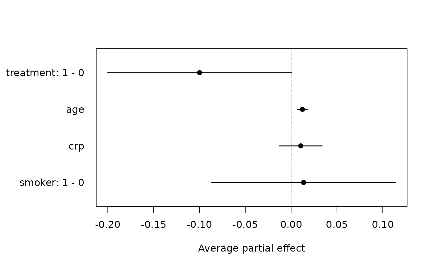
Dot-and-whisker plot of the average partial effects returned by partialeffects(): one row per continuous or binary regressor and per non-reference factor level, the estimate as a dot, its Wald confidence interval as a horizontal segment and a dotted reference line at zero. The left margin is widened to fit the row labels and restored on exit. For two-part models the part of the mean ("total", "binary" or "positive") is shown in the axis label; plot one object per part to compare them.

Usage

# S3 method for class 'panglm_ape'
plot(x, labels = NULL, xlab = NULL, main = NULL, col = "black", pch = 19, ...)

Arguments

x

a "panglm_ape" object from partialeffects()

labels

row labels; by default the variable name for continuous regressors and "variable: contrast" for discrete ones

xlab

horizontal-axis label

main

plot title

col

colour of the dots and whiskers

pch

plotting symbol of the estimates

...

passed to graphics::plot.default()

Value

x, invisibly

See also

Other panglm methods: coefplot(), confint.panglm(), effectcurve(), fitted.panglm(), fixef(), glance.panglm(), logLik.panglm(), model.matrix.panglm(), partialeffects.panordered(), plot.panglm(), plot.panglm_effectcurve(), predict.panglm(), predict.panordered(), residuals.panglm(), summary.panglm(), tidy.panglm(), vcov.panglm()

Examples

data(copd)
fit <- panglm(hospitalized ~ treatment + age + crp + factor(smoker),
              data = copd, index = c("id", "visit"), family = "probit")
plot(partialeffects(fit))