Plot a fitted panglm model

Base-graphics coefficient and diagnostic plots of a panglm() fit.

Usage

# S3 method for class 'panglm'
plot(
  x,
  which = c("coefficients", "residuals", "fitted", "qq", "calibration", "rootogram",
    "density", "effects", "correlation"),
  level = 0.95,
  parm = NULL,
  type = c("pearson", "response"),
  bins = 10,
  max = NULL,
  bw = "nrd0",
  cells = FALSE,
  main = NULL,
  xlab = NULL,
  ...
)

Arguments

x: a fitted "panglm" object
which: one of "coefficients", "residuals", "fitted", "qq", "calibration", "rootogram", "density", "effects" or "correlation"
level: confidence level for coefficient and calibration intervals
parm: names or positions of the terms of the coefficient and correlation plots; by default every term except "(Intercept)"
type: residuals of the "residuals" view, "pearson" (default) or "response"
bins: number of quantile bins of the calibration plot
max: largest count of the rootogram; by default the 99th percentile of the outcome
bw: bandwidth of the kernel densities of the "density" and "effects" views, passed to stats::density()
cells: for "correlation", print the correlation in each cell
main: optional plot title
xlab: optional horizontal-axis label
...: additional arguments passed to graphics::plot.default()

Value

x, invisibly

Details

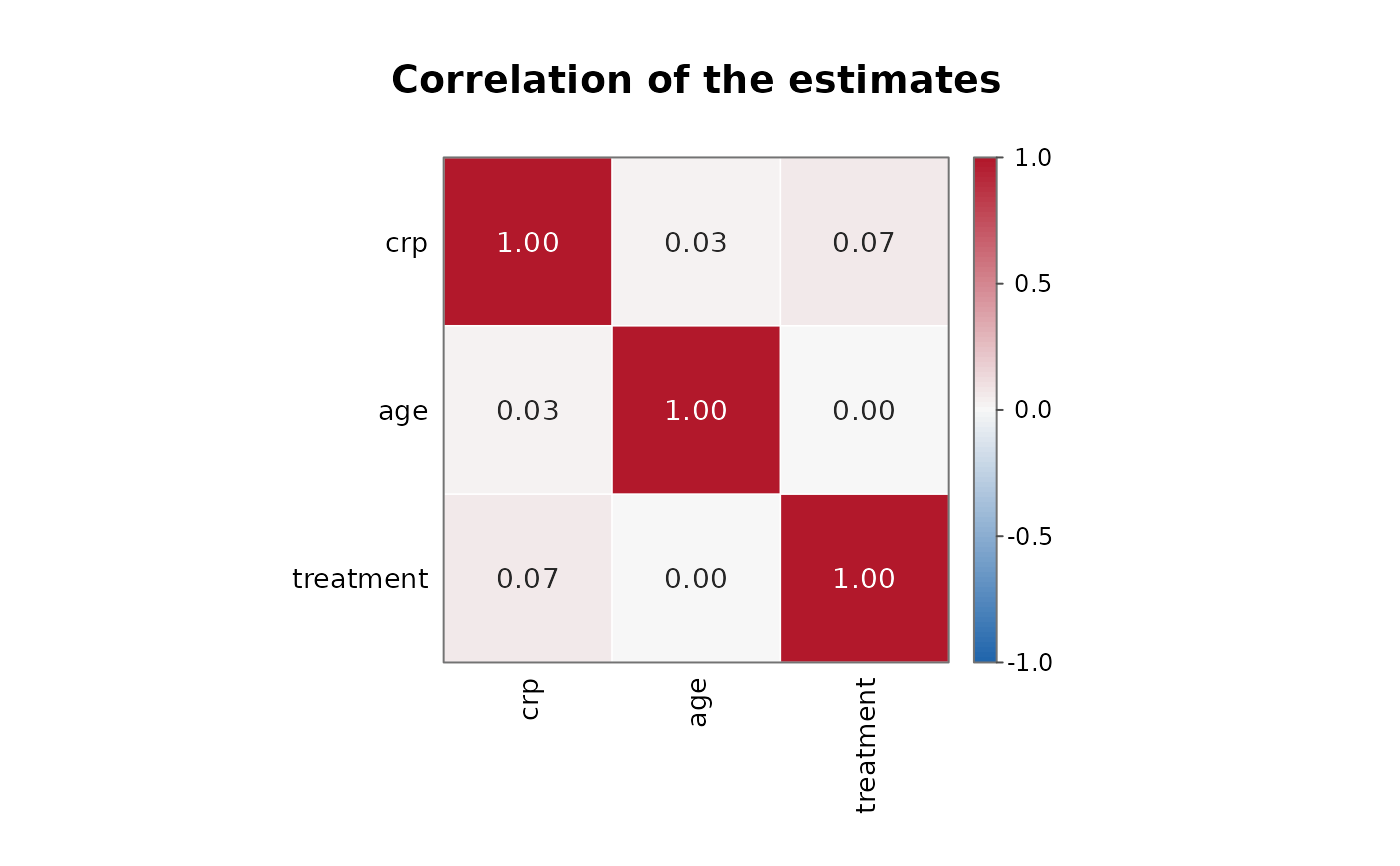
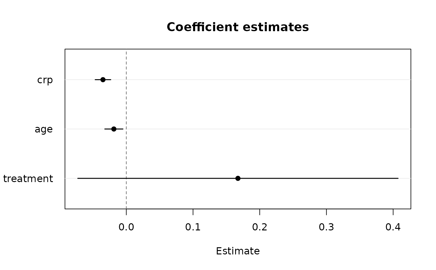
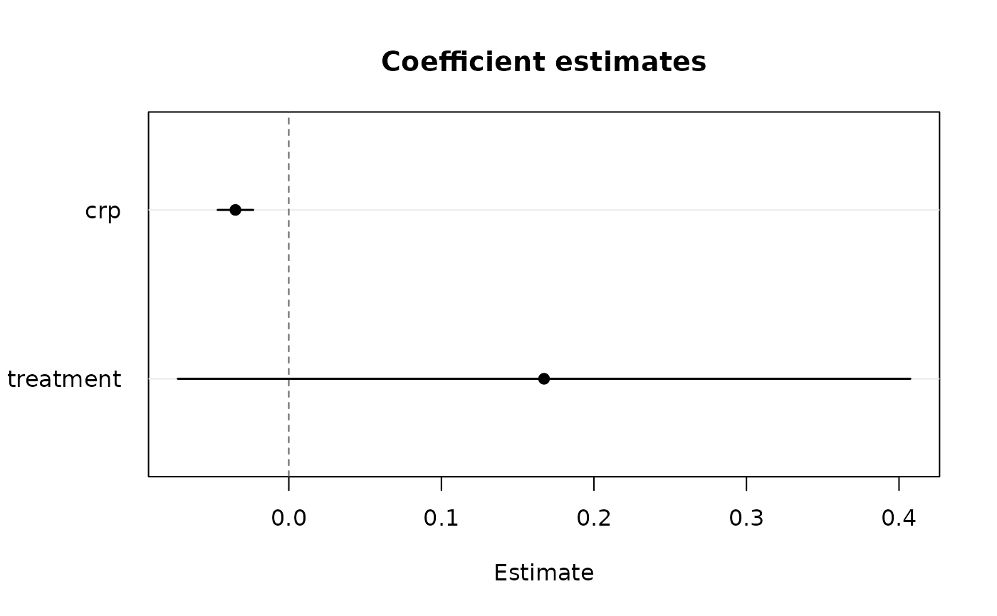
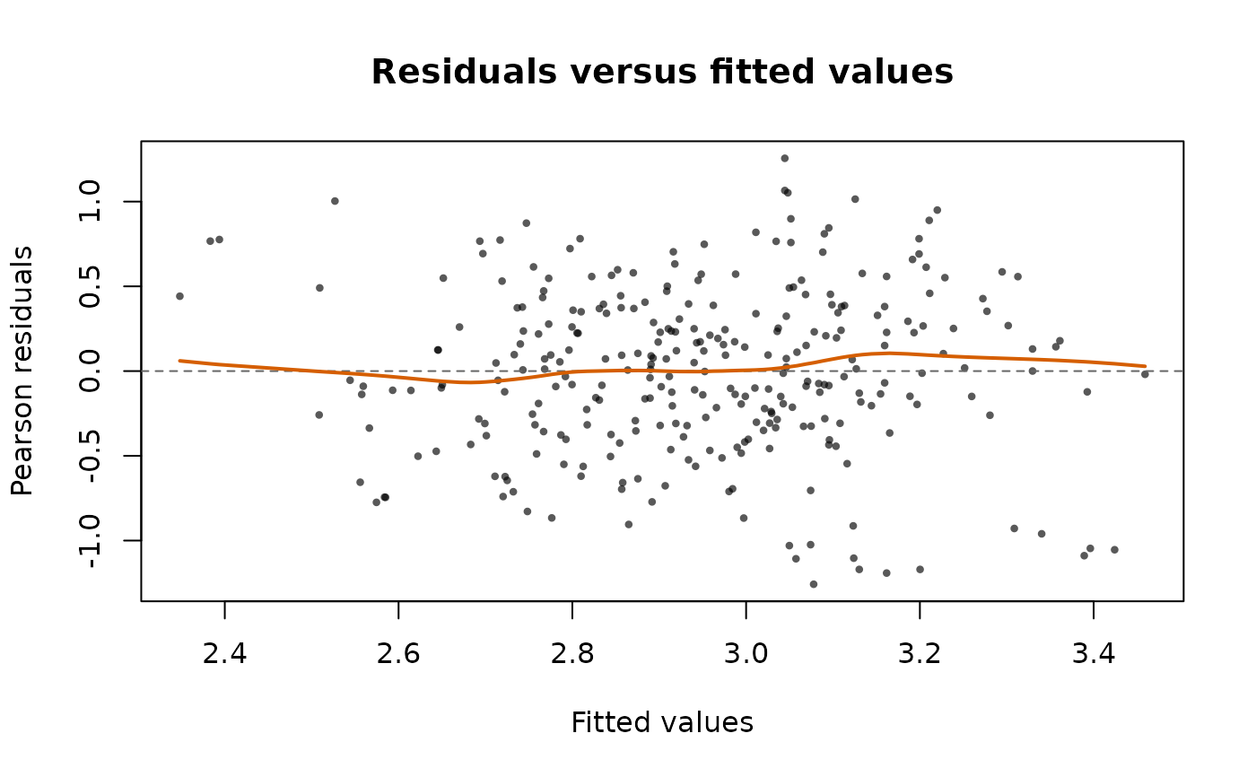
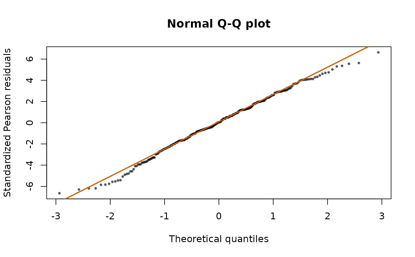
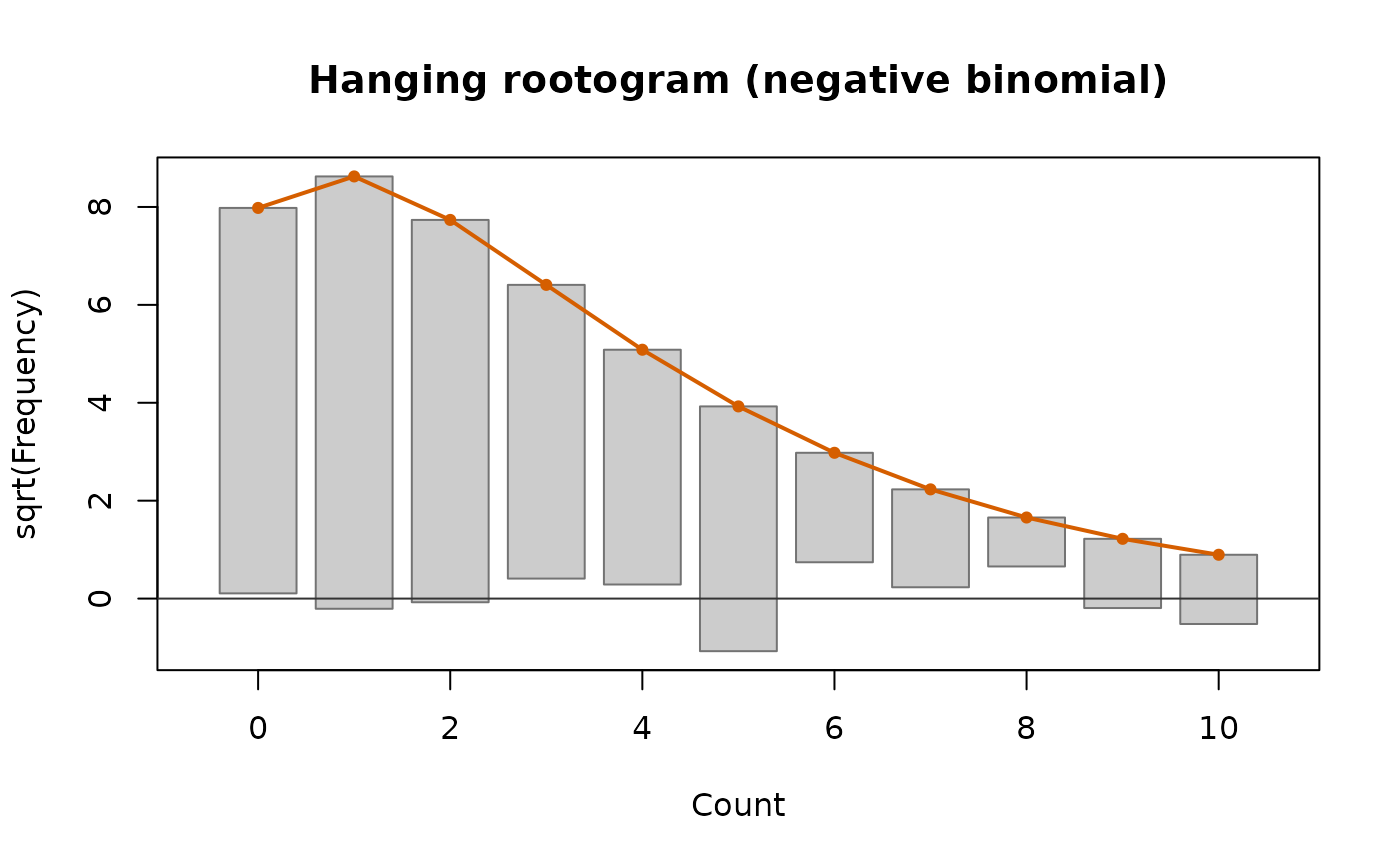
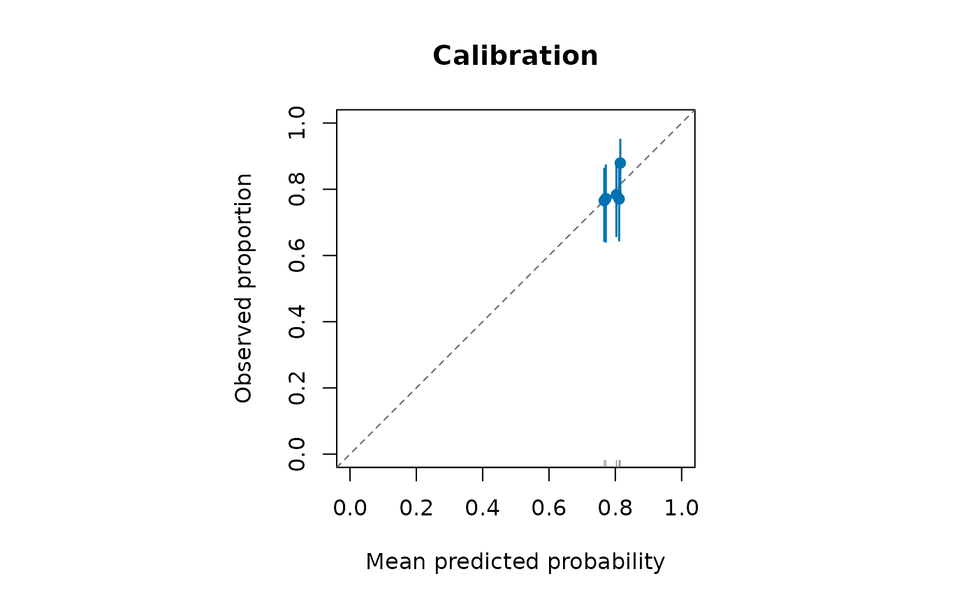
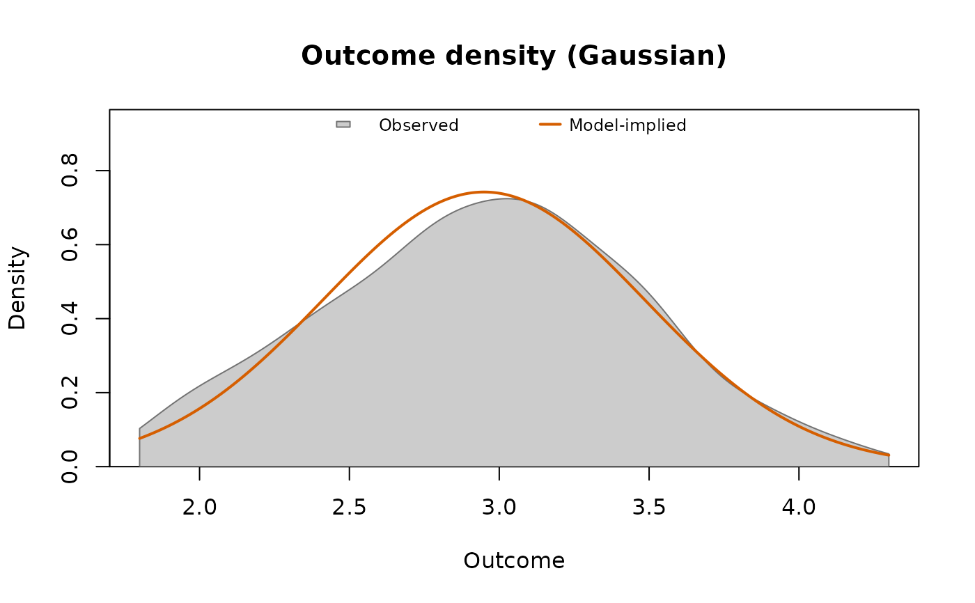
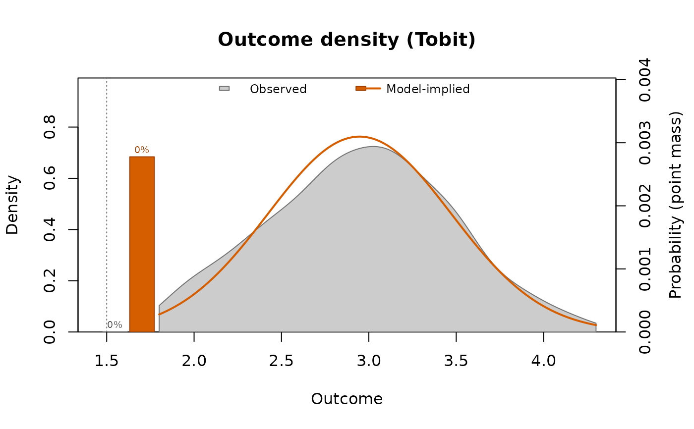
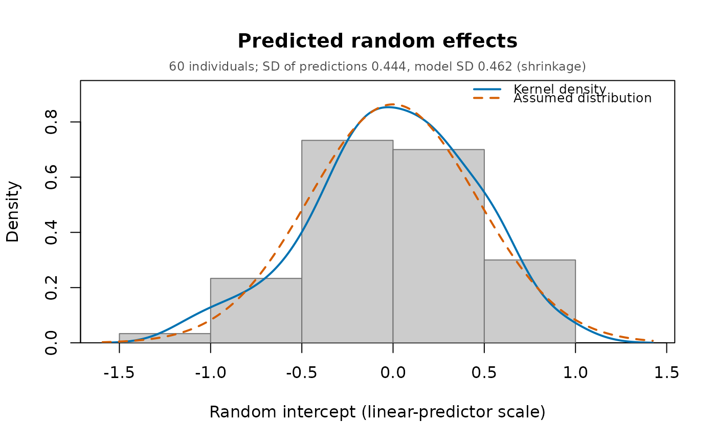
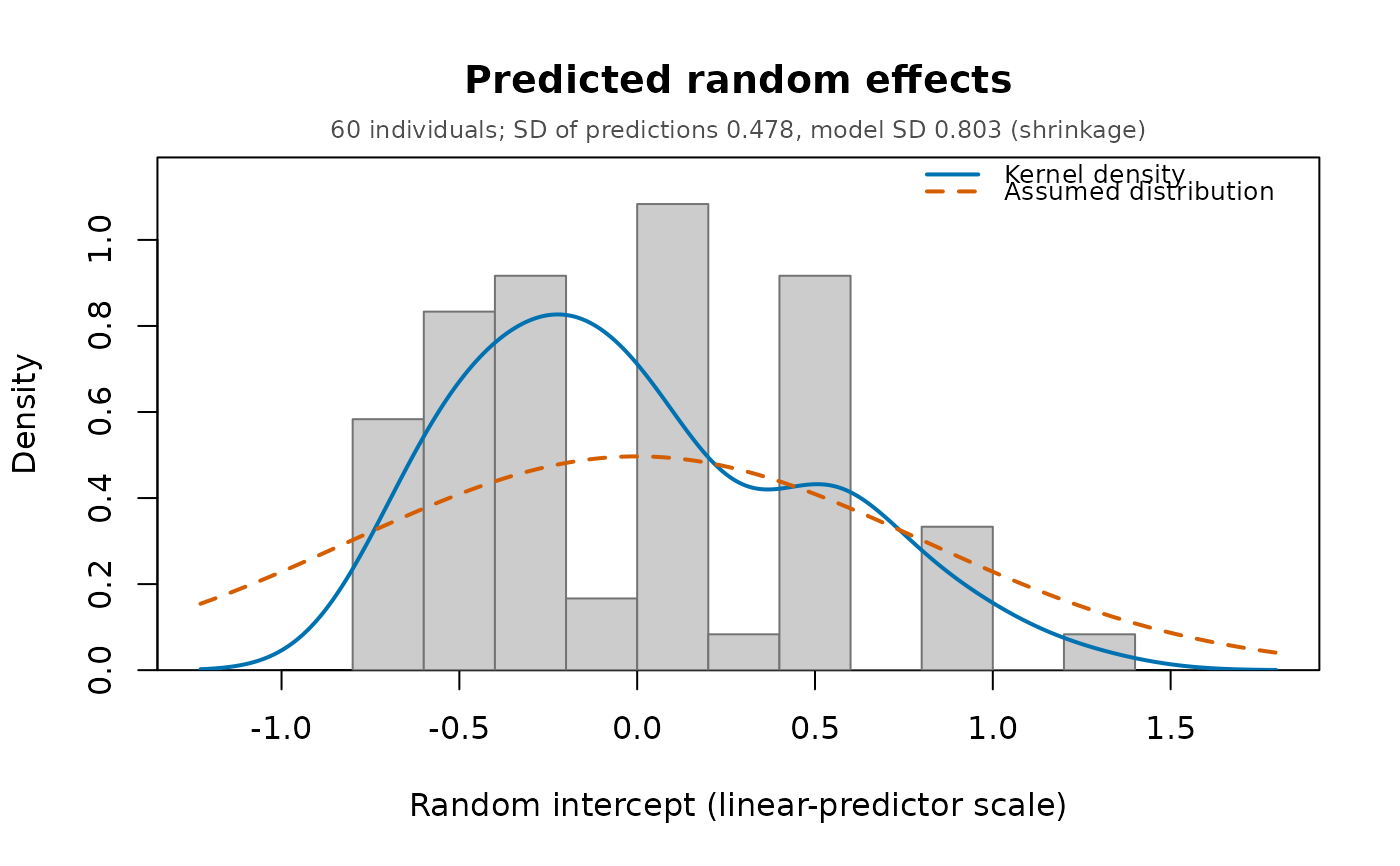
"coefficients": estimates with Wald confidence intervals (the dot-and-whisker layout shared by every panglm coefficient plot and by coefplot()); the left margin is sized to the longest term label.
"residuals": residuals against fitted values with a stats::lowess() smooth. Pearson residuals by default (see residuals.panglm() for the variance functions); for the ordered and Tobit families, where they are not defined, response residuals are drawn with a message. For log-link families (Poisson, negative binomial, log-link gamma) the fitted values are on a logarithmic axis, which spreads the many small means of count data.
"fitted": observed against fitted values with the 45-degree line.
"qq": normal Q-Q plot of the Pearson residuals with a reference line through the quartiles; for the Gaussian and gamma families the residuals are divided by the square root of the dispersion (standardized Pearson residuals). For discrete outcomes the plot is lumpy by construction and mainly shows skewness and outliers.
"calibration" (binomial families, logit or probit): observed proportion against mean predicted probability in bins quantile bins of the predicted probability, with exact (Clopper-Pearson) binomial confidence intervals and the 45-degree line.
"rootogram" (Poisson and negative binomial families): hanging rootogram. The curve is sqrt(E_k), the expected frequency of count k summed over observations, E_k = sum_i P(y_i = k); the bars of height sqrt(O_k) (observed frequency) hang from it, so that bars ending above zero mark counts predicted too often and bars ending below zero counts predicted too rarely. P(y_i = k) is the Poisson or NB2 probability at the fitted mean for pooled and fixed-effects fits (the fixed-effects means include the estimated individual effects). For random-intercept fits it is the marginal probability of a single observation implied by the mixing distribution, which is exactly the distribution whose frequencies the rootogram compares: negative binomial with size d for the Poisson-gamma model, beta-negative binomial for the Hausman-Hall-Griliches negative binomial model. Random-slope fits have no closed-form marginal and are not supported.
"density" (Gaussian, gamma, beta and Tobit families): the kernel density of the observed outcome (stats::density(), bandwidth bw, grey) against the model-implied marginal density (orange), the average over observations of the density of a single outcome at the fitted parameters, f(t) = mean_i f(t | x_i). Gaussian: dnorm(t, eta_i, sigma) with sigma^2 the residual variance; gamma: dgamma(t, shape = 1 / phi, rate = 1 / (phi mu_i)) with phi the Pearson dispersion of the fit (the stats::glm() convention, also used in the paper); beta: dbeta(t, mu_i phi, (1 - mu_i) phi) with phi the precision; Tobit: the normal density on (left, right) plus point masses P(y = left) = mean_i pnorm((left - eta_i) / sigma) (and likewise at right), drawn as bars on the right-hand axis, observed share (grey) beside predicted probability (orange). For the Tobit family the observed kernel density uses the uncensored outcomes and is scaled by their share, so that both curves integrate with the masses to one. Random-effects fits use the marginal density, integrated over the random effect: in closed form for the Gaussian and Tobit families (variance sigma_e^2 + sigma_u^2, or sigma_e^2 + z' Sigma z with random slopes) and by Gauss-Hermite quadrature (at least 21 nodes) for the gamma and beta families (the gamma random-intercept fit uses its maximum likelihood shape). Fixed-effects fits condition on the estimated individual effects (the fitted means include them), so the implied density is the in-sample fit with n + G parameters; between fits are refused. A positive outcome whose 99th percentile exceeds 20 times its median is drawn on a logarithmic axis (log = "x" forces it, log = "" turns it off): both curves are then densities of log(y), the implied one exp(s) f(exp(s)), and point masses at zero sit left of the axis. Count families are refused in favour of which = "rootogram".
"effects": distribution of the estimated individual effects. Fixed-effects fits: histogram and kernel density (blue) of fixef(). Random-effects fits: histogram and kernel density of the posterior means ranef(), with the assumed distribution of the random effect (dashed orange): N(0, sigma_u^2) for the normal random intercepts, the log-gamma density of log(nu) for the Poisson-gamma model and the logistic-beta density of log(delta) for the Hausman-Hall-Griliches negative binomial model. Empirical Bayes predictions are shrunk towards their mean, so the histogram is narrower than the assumed density; the subtitle compares the standard deviation of the predictions with the model one. A histogram much narrower than the curve signals little information per individual, not misspecification; marked skewness or several modes do suggest a non-normal effect distribution. With random slopes there is one panel per effect, then the intercept plotted against each slope with the 95% contour of the estimated normal distribution.
"correlation": heatmap of the correlation matrix of the estimates, cov2cor(vcov(x)), with a diverging palette centred at zero (blue negative, red positive, on the fixed range [-1, 1]) and a colour key; cells = TRUE prints the values. Strong correlations flag nearly collinear terms whose separate estimates are imprecise. parm selects the terms (by default all except "(Intercept)").

Examples

data(copd)
fit <- panglm(fev1 ~ crp + age + treatment, data = copd,
              index = c("id", "visit"), model = "random",
              family = "gaussian")
plot(fit)

plot(fit, parm = c("crp", "treatment"))

plot(fit, which = "residuals")

plot(fit, which = "qq")


counts <- panglm(exacerbations ~ crp + treatment, data = copd,
                 index = c("id", "visit"), model = "pooling",
                 family = "negbin")
plot(counts, which = "rootogram")


any_exacerbation <- panglm(I(exacerbations > 0) ~ crp + treatment,
                           data = copd, index = c("id", "visit"),
                           model = "pooling", family = "binomial")
plot(any_exacerbation, which = "calibration", bins = 5)


plot(fit, which = "density")

censored <- panglm(pmax(fev1, 1.5) ~ crp + treatment, data = copd,
                   index = c("id", "visit"), model = "pooling",
                   family = tobitfamily(left = 1.5))
plot(censored, which = "density")


plot(fit, which = "effects")

hosp <- panglm(hospitalized ~ crp + treatment, data = copd,
               index = c("id", "visit"), model = "random",
               family = "binomial")
plot(hosp, which = "effects")


plot(fit, which = "correlation", cells = TRUE)

Usage

Arguments

Value

Details

See also

Examples