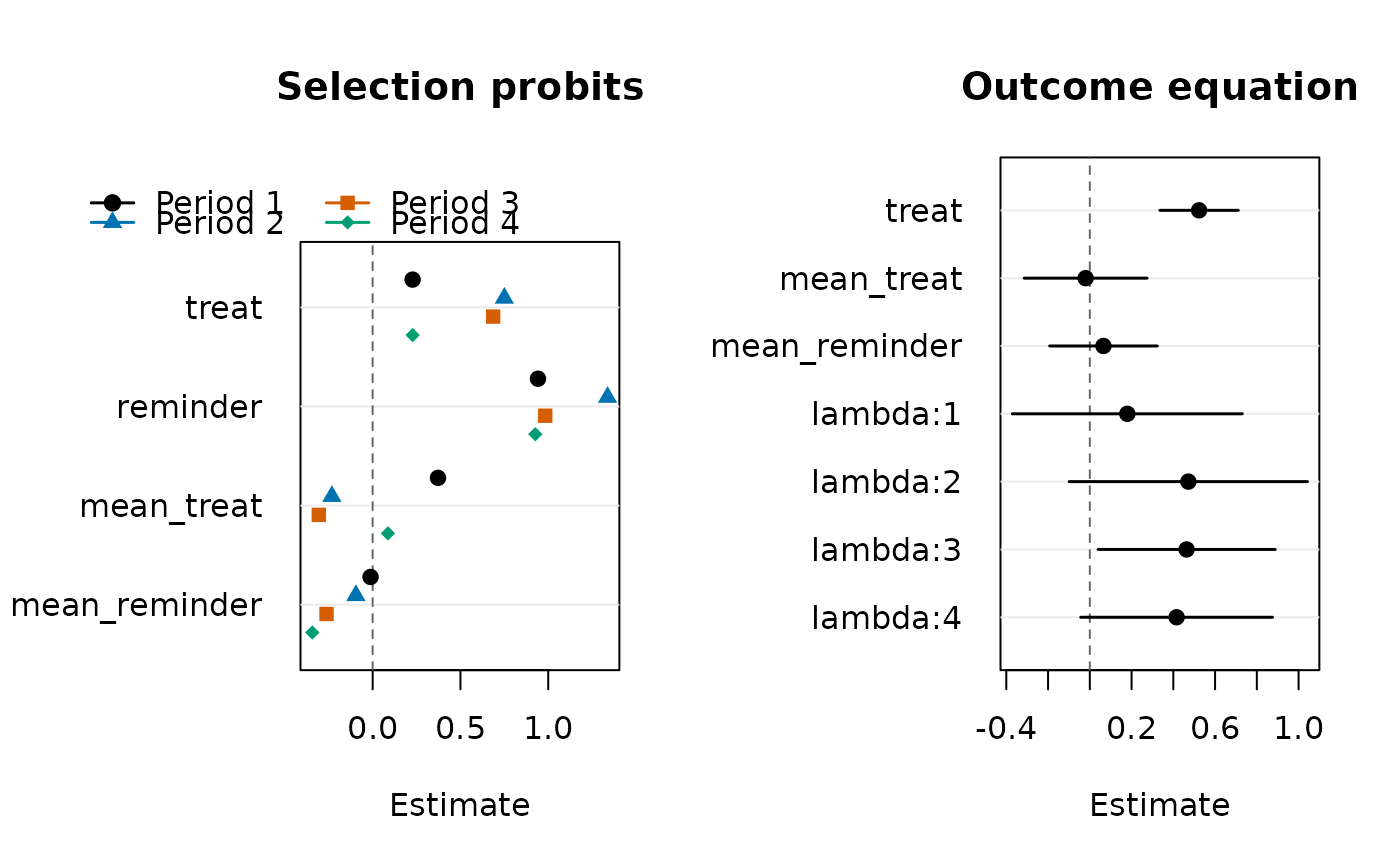
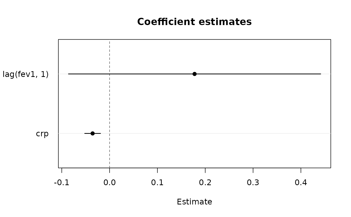
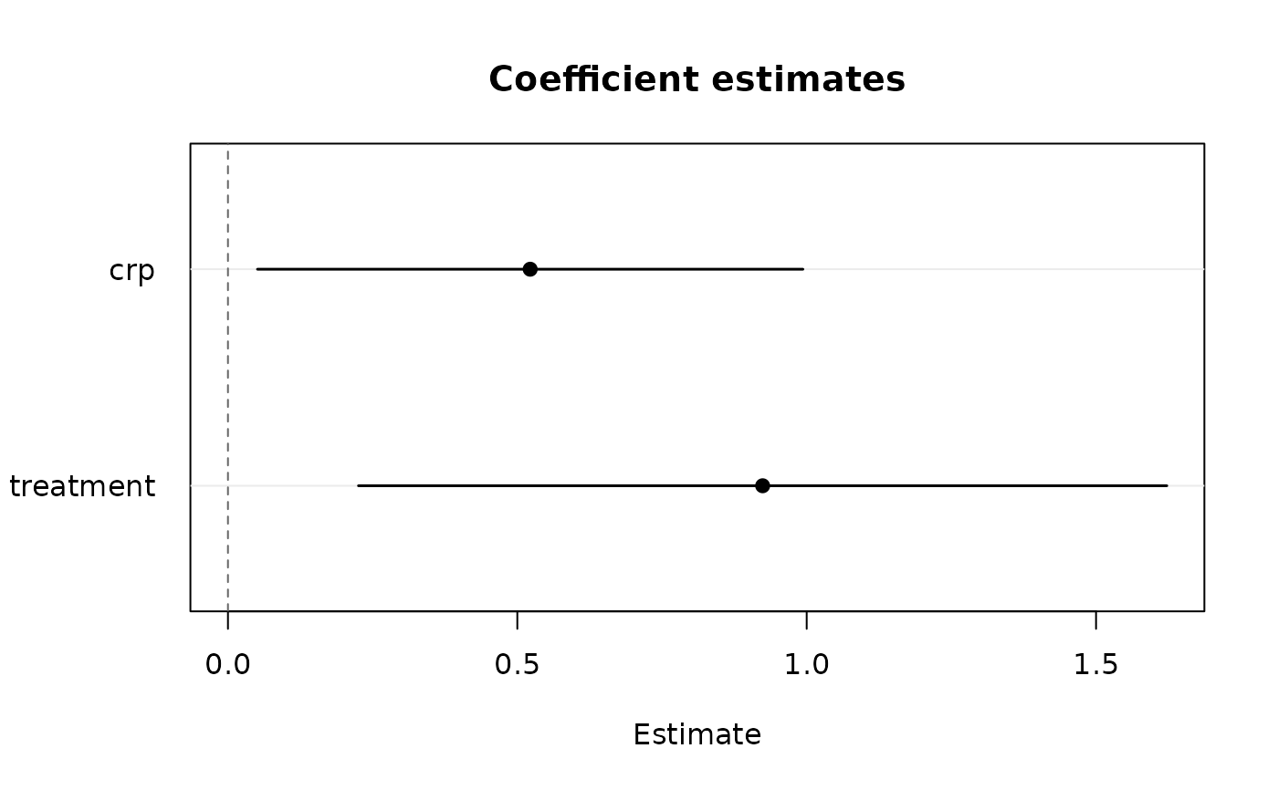
Coefficient estimates with Wald confidence intervals, in the
dot-and-whisker layout of plot.panglm(). For panselect() fits,
which = "selection" shows the coefficients of the per-period probits of
the selection equation (one marker per period, dodged within each term);
they are drawn without intervals because the first-step probits are
stored without standard errors. which = "both" shows the selection and
outcome equations side by side.
Usage
# S3 method for class 'pangmm'
plot(x, parm = NULL, level = 0.95, main = NULL, xlab = NULL, ...)

# S3 method for class 'paniv'
plot(x, parm = NULL, level = 0.95, main = NULL, xlab = NULL, ...)

# S3 method for class 'panselect'
plot(
  x,
  which = c("both", "outcome", "selection"),
  parm = NULL,
  level = 0.95,
  xlab = NULL,
  ...
)
Arguments
- x
a fitted
"pangmm","paniv"or"panselect"object- parm
names or positions of the terms to plot; by default every term except
"(Intercept)"- level
confidence level of the intervals
- main
optional plot title
- xlab
optional horizontal-axis label
- ...
additional arguments passed to
graphics::plot.default()- which
for
panselectfits,"both"(default),"outcome"or"selection"
See also
Other pangmm methods:
predict.pangmm(),
summary.pangmm(),
vcov.pangmm()
Other paniv methods:
predict.paniv(),
summary.paniv(),
vcov.paniv()
Other panselect methods:
predict.panselect(),
summary.panselect(),
vcov.panselect()
Examples
data(copd)
gm <- pangmm(fev1 ~ lag(fev1, 1) + crp | lag(fev1, 2:99), data = copd,
index = c("id", "visit"))
plot(gm, parm = c("lag(fev1, 1)", "crp"))
 iv <- paniv(fev1 ~ crp + treatment | age + treatment, data = copd,
index = c("id", "visit"), model = "pooling")
plot(iv)
 set.seed(1)
d <- data.frame(id = rep(1:150, each = 4), wave = rep(1:4, 150))
d$treat <- rnorm(600)
d$reminder <- rnorm(600)
v <- rnorm(600)
d$respond <- as.numeric(0.3 + 0.5 * d$treat + d$reminder + v > 0)
d$qol <- ifelse(d$respond == 1, 1 + 0.5 * d$treat + 0.7 * v + rnorm(600), NA)
sel <- panselect(respond ~ treat + reminder, qol ~ treat, data = d,
index = c("id", "wave"), model = "pooling", boot = 0)
plot(sel)