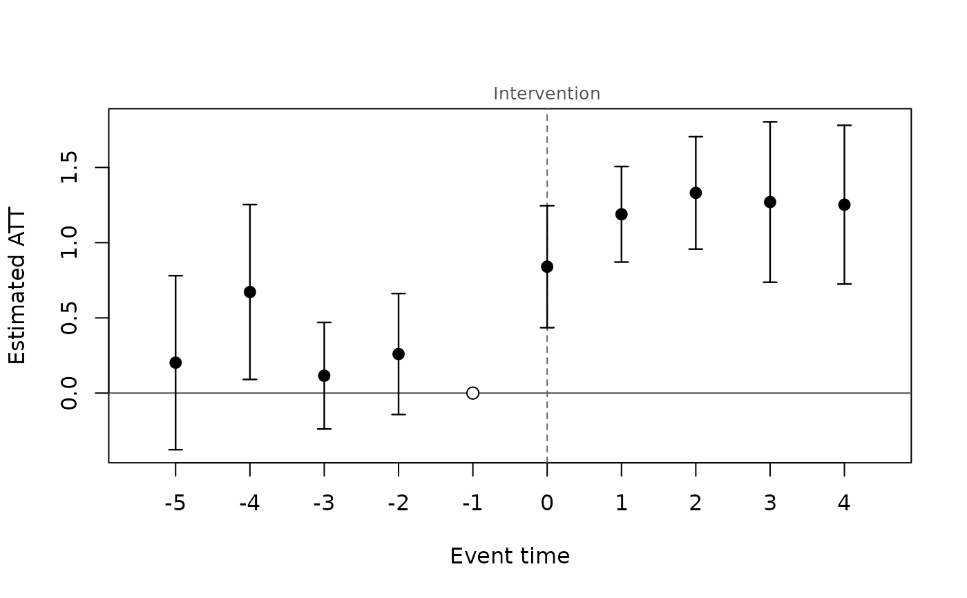
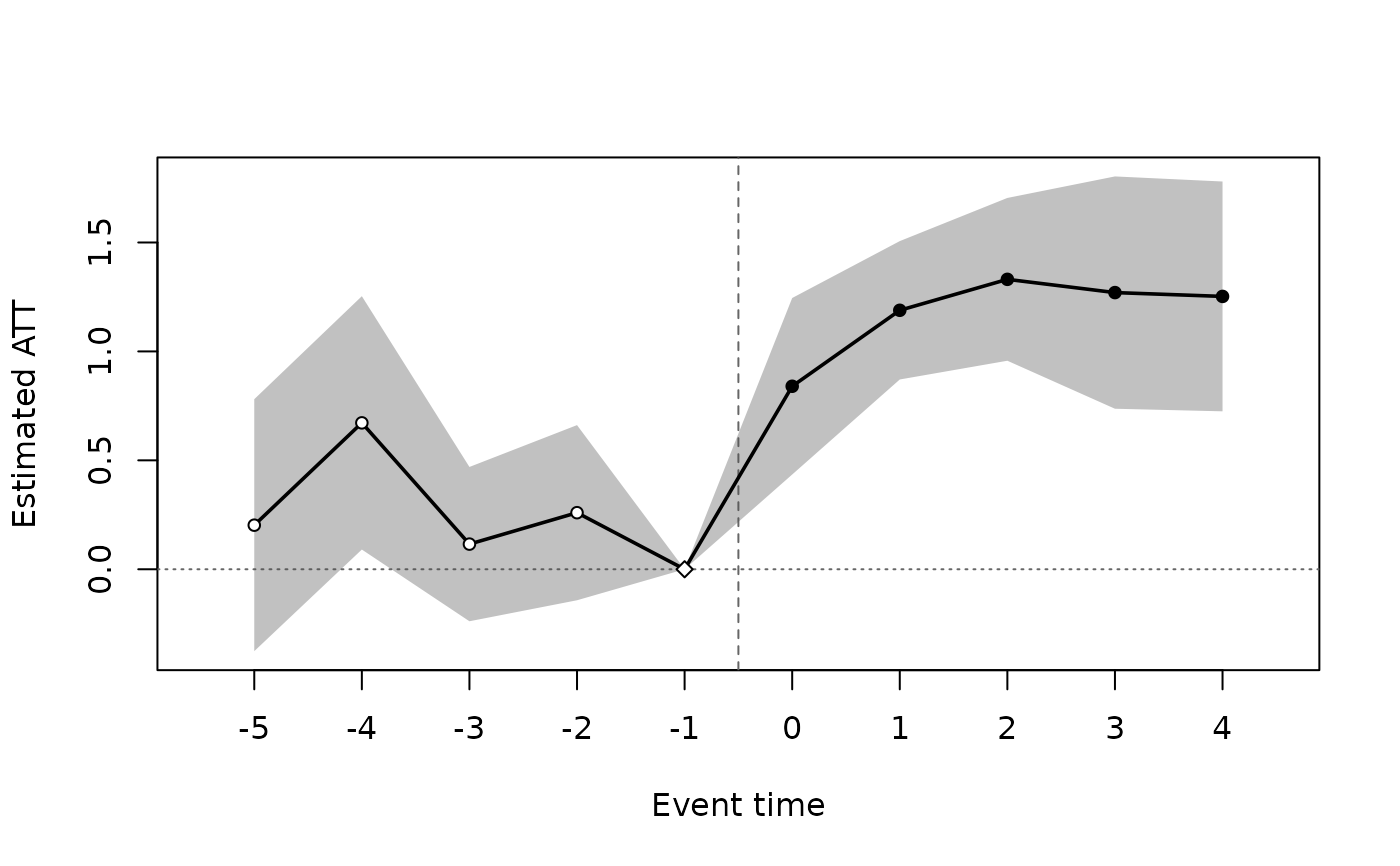
Plots the event-study aggregation of an etwfe() fit (or the cohort or
calendar aggregation) with pointwise confidence intervals, in the
styles of plot.panglm_attgt() (see its Styles section). The reference
period (event time -1 with control = "never") is drawn as an open
symbol at zero.
Usage
# S3 method for class 'panglm_etwfe'
plot(
  x,
  type = c("event", "group", "calendar", "heatmap"),
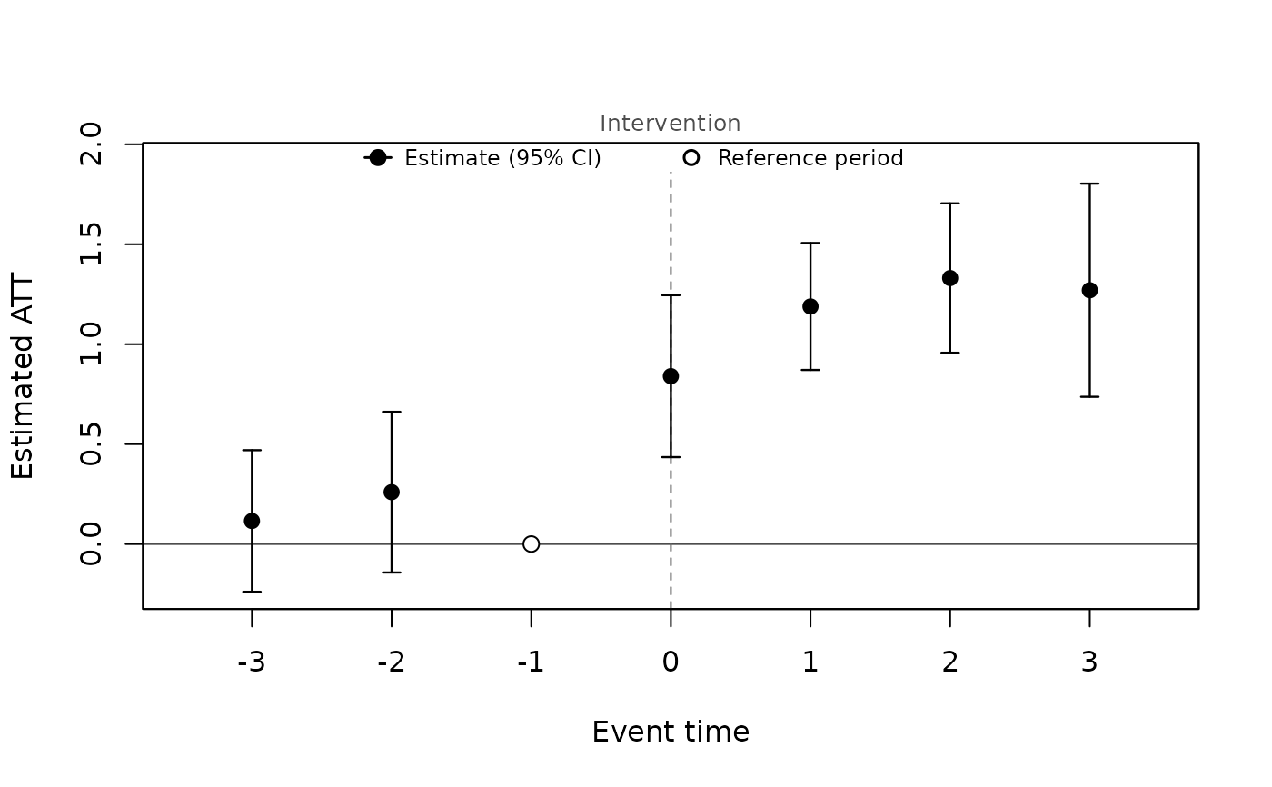
  min_e = -Inf,
  max_e = Inf,
  xlab = NULL,
  ylab = "Estimated ATT",
  main = NULL,
  ylim = NULL,
  legend = FALSE,
  style = c("classic", "points", "line"),
  ref = -1,
  onset = NULL,
  onset_label = NA,
  caps = NULL,
  cells = FALSE,
  digits = 2,
  ...
)

# S3 method for class 'summary.panglm_etwfe'
plot(
  x,
  type = NULL,
  min_e = -Inf,
  max_e = Inf,
  xlab = NULL,
  ylab = "Estimated ATT",
  main = NULL,
  ylim = NULL,
  legend = FALSE,
  style = c("classic", "points", "line"),
  ref = -1,
  onset = NULL,
  onset_label = NA,
  caps = NULL,
  ...
)
Arguments
- x
a
"panglm_etwfe"fit frometwfe(), or its summary- type
aggregation to plot (for a fit):
"event","group","calendar"or"heatmap"(cohort by period heat map of ATT(g, t))- min_e, max_e
event window to plot (event time for the event-time plot, calendar time for the heat map)
- xlab, ylab, main
axis labels and title
- ylim
y-axis limits
- legend
logical: add a compact legend of the symbols
- style
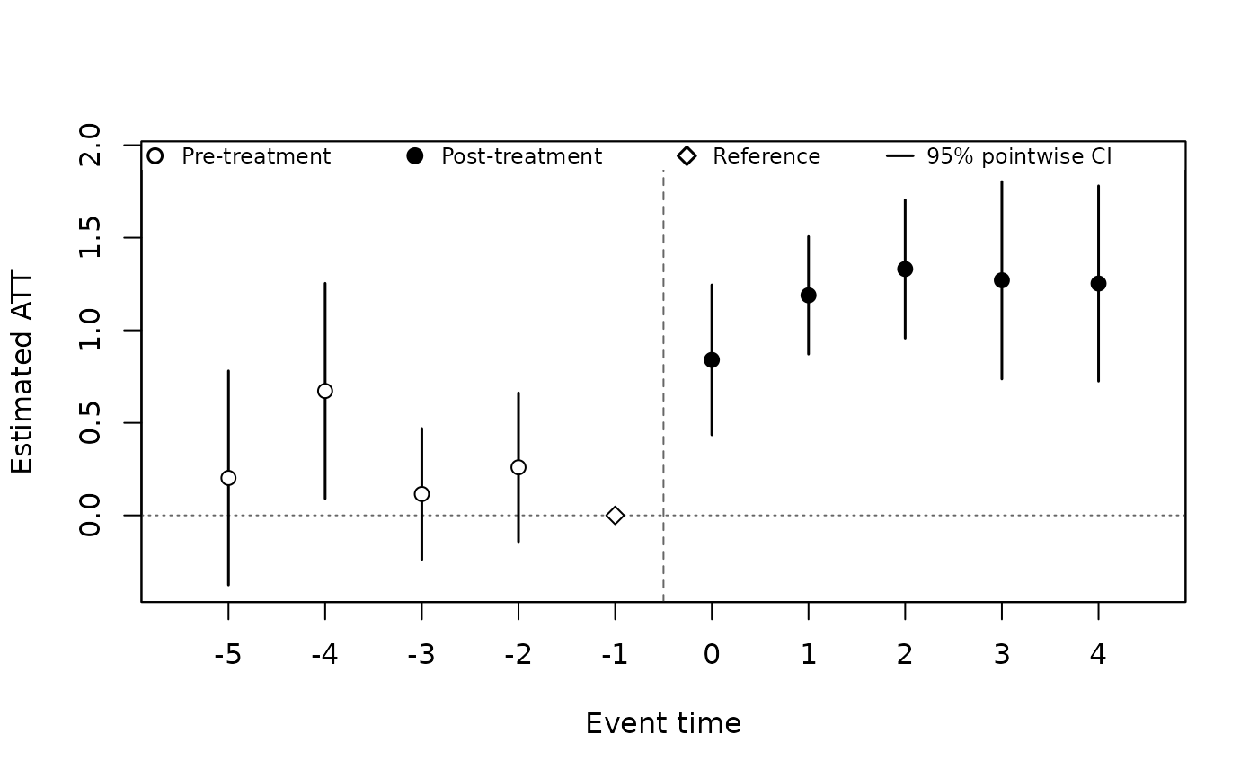
"classic"(default),"points"or"line"(see Styles); for the event-time, cohort and calendar plots- ref
event time of the reference period, marked when its estimate is exactly zero: event time
-1withcontrol = "never"; withcontrol = "notyet"there are no pre-treatment effects- onset
position of the dashed treatment-onset line on the event time axis:
NULLgives0forstyle = "classic"and-0.5(between the last pre-treatment and the first treated period) otherwise- onset_label
text written above the onset line; the default (
NA) is "Intervention" forstyle = "classic"and none otherwise,NULLsuppresses it- caps
logical: draw caps on the confidence-interval whiskers; the default (
NULL) draws them forstyle = "classic"only- cells
logical: print the estimates in the cells of the heat map
- digits
number of decimals of the printed estimates
- ...
passed to
graphics::plot()
Value
the plotted summary, invisibly; for the heat map, the table of
ATT(g, t) with a logical column pre (pre-treatment cell)
Details
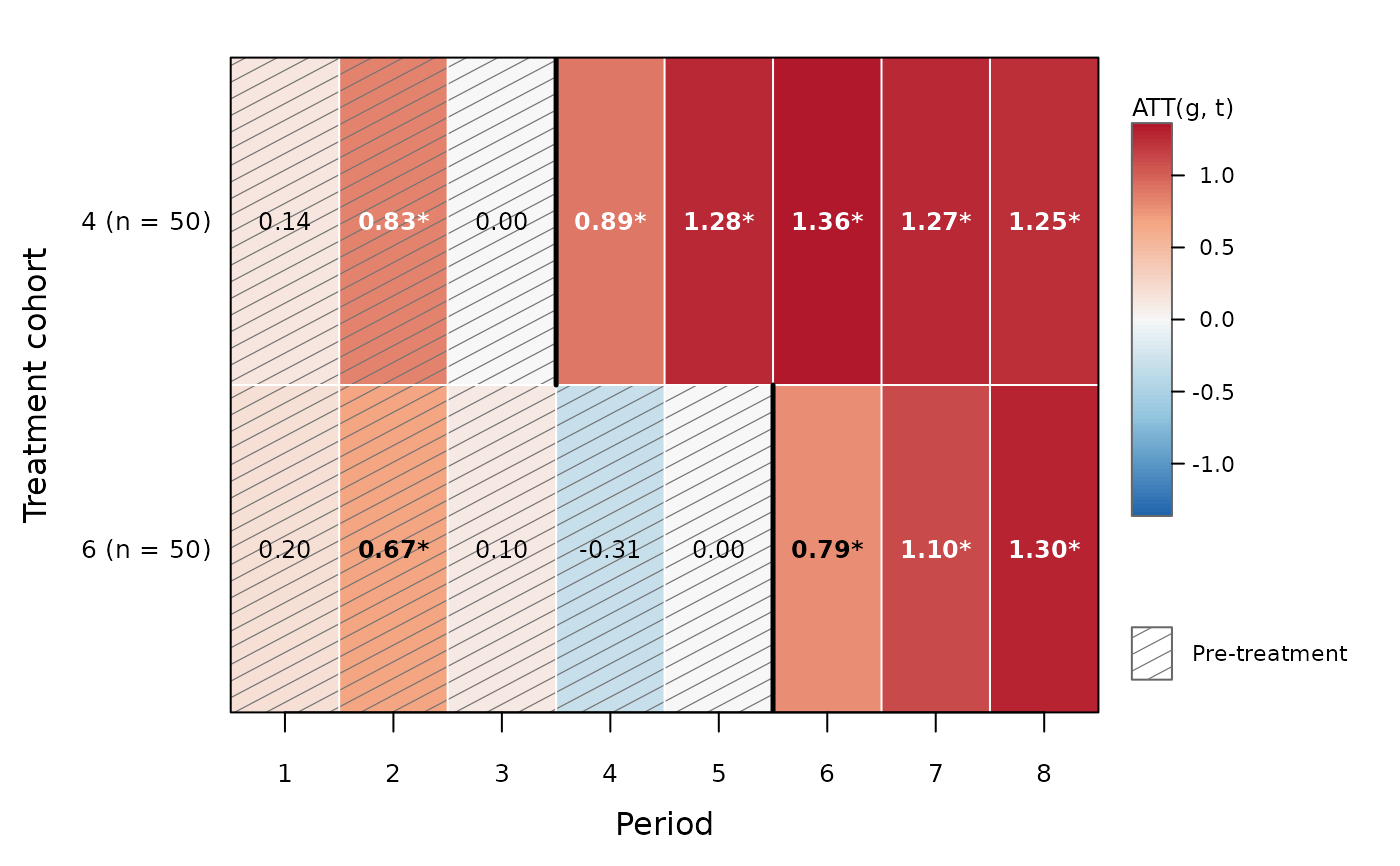
type = "heatmap" draws the cohort-by-period effects ATT(g, t) on the
response scale as a heat map, as for plot.panglm_attgt(); with
control = "never" the reference cell g - 1 of each cohort is zero.
See also
Other etwfe methods:
summary.panglm_etwfe()
Examples
set.seed(2)
d <- expand.grid(id = 1:150, t = 1:8)
d$first <- rep(c(4, 6, NA), each = 50)[d$id]
d$y <- rnorm(150)[d$id] + 0.2 * d$t +
ifelse(!is.na(d$first) & d$t >= d$first, 1, 0) + rnorm(nrow(d))
fit <- etwfe(y ~ 1, d, index = c("id", "t"), treat = "first", control = "never")
plot(fit)
 plot(fit, min_e = -3, max_e = 3, legend = TRUE)
 plot(fit, style = "points", legend = TRUE)
 plot(fit, style = "line")
 plot(fit, type = "heatmap", cells = TRUE)