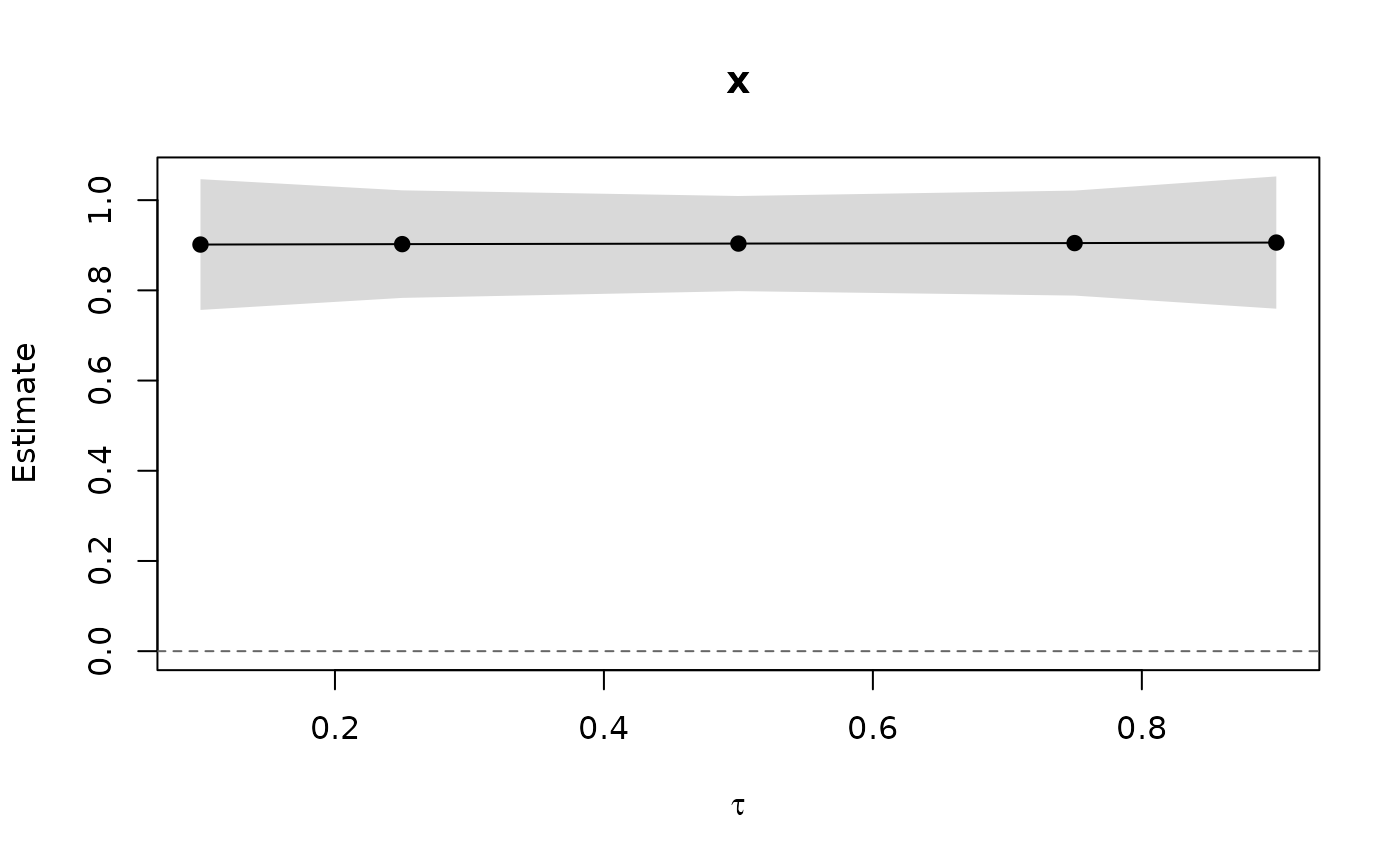
Base-graphics plot of the coefficients of a panqr() fit across the
estimated quantiles, one panel per term: the estimates joined by a line,
a shaded pointwise Wald confidence band (from the same variances as
confint()), and a dashed reference line at zero. With a single quantile
each panel shows the estimate and its interval. Without a covariance
(vcov = "none") only the estimates are drawn.
Usage
# S3 method for class 'panqr'
plot(
  x,
  parm = NULL,
  level = 0.95,
  ncol = NULL,
  col = "black",
  band = "grey85",
  main = NULL,
  xlab = expression(tau),
  ylab = "Estimate",
  ...
)
Arguments
- x
a
"panqr"fit- parm
names or positions of the terms to plot; all by default
- level
confidence level of the bands
- ncol
number of panel columns; by default up to three
- col
colour of the estimates
- band
colour of the confidence bands
- main
optional titles, recycled over the terms; the term names by default
- xlab
horizontal-axis label
- ylab
vertical-axis label
- ...
additional arguments passed to
graphics::plot.default()
See also
Other panqr methods:
summary.panqr(),
vcov.panqr()
Examples
set.seed(2)
d <- data.frame(id = rep(1:100, each = 5), t = rep(1:5, 100))
d$x <- rnorm(500) + rep(rnorm(100), each = 5)
d$y <- d$x + rep(rnorm(100), each = 5) + (1 + 0.2 * abs(d$x)) * rnorm(500)
fit <- panqr(y ~ x, data = d, index = c("id", "t"),
             tau = c(0.1, 0.25, 0.5, 0.75, 0.9), model = "mmqr")
plot(fit)