basetable: A Tutorial

A walk through the package README, with more examples for every verb family

packages

tutorial

Author

Imad El Badisy

Published

September 5, 2026

I get more questions about how to actually use basetable day to day than about anything in the benchmarks, so this post takes the README and adds worked examples for the handful of functions that carry most of the day-to-day work and the performance story: subset(), transform(), aggregate(), merge() / semimerge(), and describe(). The README itself is unchanged below - the new material is the “Tutorial” section in the middle, and the figures and tables in “Performance” are exactly as published, with a link to the script that generated them.

basetable

basetable is a fast in-memory data-manipulation package for R with a base-R interface and no dependencies. You write subset(), transform(), aggregate(), merge(), split(), and the work runs on the package’s own C++ engine. There is no data.table, no dplyr, no Arrow underneath, and nothing in Imports beyond the base and recommended packages (parallel, stats, utils).

Every verb returns a basetable: an ordinary data.frame with one extra class so it prints compactly and [ keeps the class. as.data.frame() strips it back to a plain frame.

This is a deliberately focused tool. It is aimed at

people teaching or learning base R who want speed without the cognitive load of tidy evaluation or [i, j, by], and
codebases already built on subset() / merge() / aggregate() that want a faster engine without a rewrite.

Design

Base-style naming and semantics. Functions read like subset(), transform(), aggregate(), merge(), split().
A native C++ engine. Projection, filtering, ordering, distinct, grouping, all join kinds, row-bind and subset() predicate evaluation run in compiled .Call kernels. There is no third-party compute backend.
Explicit, standard-evaluation interfaces. Column names are strings, not captured symbols (with the marked exceptions subset() and transform() inherit from base R).
Zero hard dependencies. data.table and dplyr appear only in Suggests, and only as competitors in the benchmark vignette.

Installation

# install.packages("pak")
pak::pak("ielbadisy/basetable")

Minimal examples

# nested
basetable::describe(
  basetable::transform(
    basetable::subset(mtcars, cyl == 6, select = c("mpg", "hp", "wt", "cyl")),
    power = hp / wt
  )
)

# basetable: 5 x 14
  column   class n missing missing_prop distinct       mean         sd
1    mpg numeric 7       0            0        6  19.742857  1.4535670
2     hp numeric 7       0            0        4 122.285714 24.2604911
3     wt numeric 7       0            0        6   3.117143  0.3563455
4    cyl numeric 7       0            0        1   6.000000  0.0000000
5  power numeric 7       0            0        6  39.927938 10.8533912
        min       q25    median      q75      max top
1  17.80000  18.65000  19.70000  21.0000  21.4000    
2 105.00000 110.00000 110.00000 123.0000 175.0000    
3   2.62000   2.82250   3.21500   3.4400   3.4600    
4   6.00000   6.00000   6.00000   6.0000   6.0000    
5  30.34682  34.98522  35.75581  40.1228  63.1769

# pipe
mtcars |>
  basetable::pick(c("mpg", "hp", "wt", "cyl")) |>
  basetable::transform(power = hp / wt) |>
  basetable::aggregate(by = "cyl", value = c("mpg", "power"), fun = mean)

# basetable: 3 x 3
  cyl      mpg    power
1   4 26.66364 37.92533
2   6 19.74286 39.92794
3   8 15.10000 53.85964

# table-1 style summary
basetable::summarytab(
  basetable::transform(mtcars, am = factor(am, labels = c("Automatic", "Manual"))),
  vars = c("mpg", "hp"), by = "am", p_value = TRUE
)

# basetable: 2 x 6
  variable     level    Automatic       Manual      Overall p_value
1      mpg Mean (SD)   17.1 (3.8)   24.4 (6.2)   20.1 (6.0) 0.00137
2       hp Mean (SD) 160.3 (53.9) 126.8 (84.1) 146.7 (68.6)   0.221

Every call above is qualified with basetable::. That’s not just belt and braces for the README: basetable intentionally reuses the base-R names subset(), transform(), merge() and split(), and attaching it with a plain library(basetable) puts those ahead of base on the search path for the rest of the session - which can surprise other code, including tooling, that calls the base versions unqualified. Qualifying the calls, as in “Using basetable alongside dplyr and data.table” below, sidesteps that entirely.

Tutorial

The examples above are the pitch. The rest of this section is the short list of functions that carry most of the day-to-day work, one at a time.

Filtering: `subset()`

Same syntax as base::subset() - a condition on the unquoted column names, plus an optional select - running on the C++ engine instead of R:

basetable::subset(mtcars, cyl == 6 & hp > 100, select = c("mpg", "hp", "wt", "cyl"))

# basetable: 7 x 4
   mpg  hp    wt cyl
1 21.0 110 2.620   6
2 21.0 110 2.875   6
3 21.4 110 3.215   6
4 18.1 105 3.460   6
5 19.2 123 3.440   6
6 17.8 123 3.440   6
7 19.7 175 2.770   6

Creating columns: `transform()`

Adds or overwrites columns from expressions on the existing ones, and later expressions in the same call can use columns created earlier in it:

mtcars |>
  basetable::transform(power = hp / wt, efficient = mpg > mean(mpg))

# basetable: 32 x 13
    mpg cyl  disp  hp drat    wt  qsec vs am gear carb    power efficient
1  21.0   6 160.0 110 3.90 2.620 16.46  0  1    4    4 41.98473      TRUE
2  21.0   6 160.0 110 3.90 2.875 17.02  0  1    4    4 38.26087      TRUE
3  22.8   4 108.0  93 3.85 2.320 18.61  1  1    4    1 40.08621      TRUE
4  21.4   6 258.0 110 3.08 3.215 19.44  1  0    3    1 34.21462      TRUE
5  18.7   8 360.0 175 3.15 3.440 17.02  0  0    3    2 50.87209     FALSE
6  18.1   6 225.0 105 2.76 3.460 20.22  1  0    3    1 30.34682     FALSE
7  14.3   8 360.0 245 3.21 3.570 15.84  0  0    3    4 68.62745     FALSE
8  24.4   4 146.7  62 3.69 3.190 20.00  1  0    4    2 19.43574      TRUE
9  22.8   4 140.8  95 3.92 3.150 22.90  1  0    4    2 30.15873      TRUE
10 19.2   6 167.6 123 3.92 3.440 18.30  1  0    4    4 35.75581     FALSE
# 22 more rows

Grouped summaries: `aggregate()`

This is the one with the biggest gap in the benchmarks below - grouped reductions accumulate in compiled code without materialising intermediate columns, so a sd or a count by group allocates close to nothing:

basetable::aggregate(airquality, by = "Month", value = c("Ozone", "Temp"), fun = mean, na.rm = TRUE)

# basetable: 5 x 3
  Month    Ozone     Temp
1     5 23.61538 65.54839
2     6 29.44444 79.10000
3     7 59.11538 83.90323
4     8 59.96154 83.96774
5     9 31.44828 76.90000

Joins: `merge()` and `semimerge()`

merge() covers inner, left, right, and full joins through the same all / all.x / all.y arguments as base::merge(), rows come back in input order rather than sorted by key. semimerge() filters one table by matches in another without adding columns - the join-as-filter case that a plain merge() would otherwise need a follow-up subset() for:

left <- data.frame(id = 1:4, x = letters[1:4])
right <- data.frame(id = c(2, 3, 5), y = LETTERS[2:4])

basetable::merge(left, right, by = "id", all.x = TRUE)

# basetable: 4 x 3
  id x    y
1  1 a <NA>
2  2 b    B
3  3 c    C
4  4 d <NA>

basetable::semimerge(left, right, by = "id")

# basetable: 2 x 2
  id x
1  2 b
2  3 c

Exploration: `describe()` and `summarytab()`

describe() is the quick per-column numeric summary; summarytab() builds a table-1-style comparison across a grouping variable, shown already in the minimal examples above with a p-value column:

basetable::describe(mtcars)

# basetable: 11 x 14
   column   class  n missing missing_prop distinct       mean          sd
1     mpg numeric 32       0            0       25  20.090625   6.0269481
2     cyl numeric 32       0            0        3   6.187500   1.7859216
3    disp numeric 32       0            0       27 230.721875 123.9386938
4      hp numeric 32       0            0       22 146.687500  68.5628685
5    drat numeric 32       0            0       22   3.596563   0.5346787
6      wt numeric 32       0            0       29   3.217250   0.9784574
7    qsec numeric 32       0            0       30  17.848750   1.7869432
8      vs numeric 32       0            0        2   0.437500   0.5040161
9      am numeric 32       0            0        2   0.406250   0.4989909
10   gear numeric 32       0            0        3   3.687500   0.7378041
      min       q25  median    q75     max top
1  10.400  15.42500  19.200  22.80  33.900    
2   4.000   4.00000   6.000   8.00   8.000    
3  71.100 120.82500 196.300 326.00 472.000    
4  52.000  96.50000 123.000 180.00 335.000    
5   2.760   3.08000   3.695   3.92   4.930    
6   1.513   2.58125   3.325   3.61   5.424    
7  14.500  16.89250  17.710  18.90  22.900    
8   0.000   0.00000   0.000   1.00   1.000    
9   0.000   0.00000   0.000   1.00   1.000    
10  3.000   3.00000   4.000   4.00   5.000    
# 1 more rows

Performance

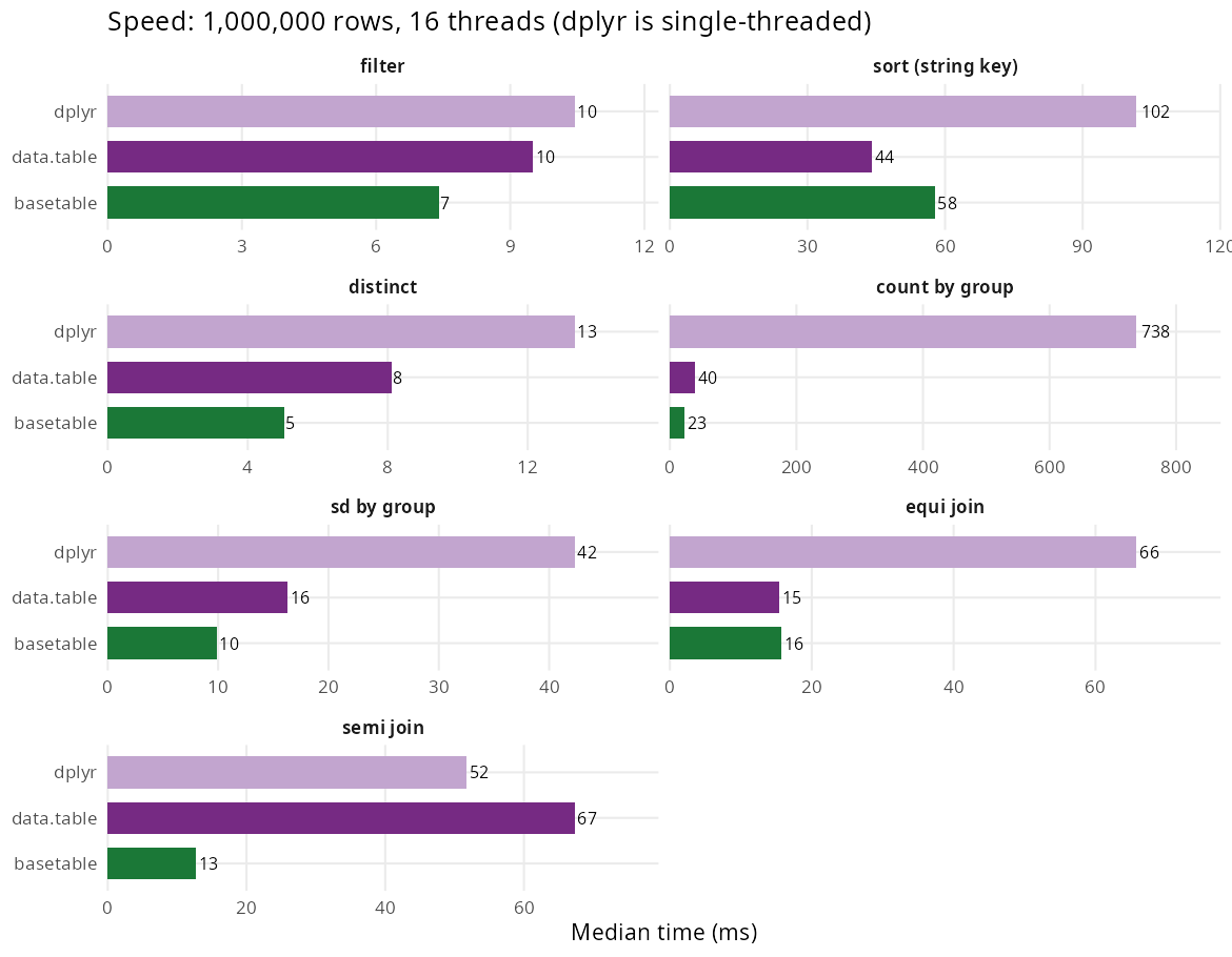
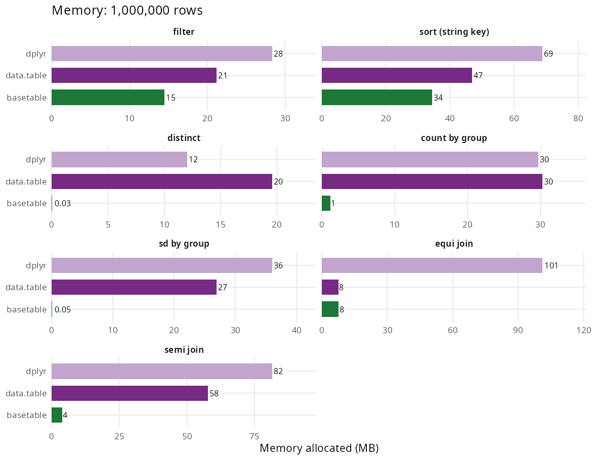
Timing and memory below come from the bench package at 1,000,000 rows on one Linux machine. The script that produced both figures and both tables is inst/benchmarks/make-readme-figures.R; the Benchmarks vignette has the full reproducible report. basetable is compared with data.table and dplyr.

Speed

Memory

Operation	basetable	data.table	dplyr	basetable mem	data.table mem	dplyr mem
filter	7 ms	10 ms	10 ms	15 MB	21 MB	28 MB
sort (string key)	58 ms	44 ms	102 ms	34 MB	47 MB	69 MB
distinct	5 ms	8 ms	13 ms	0.03 MB	20 MB	12 MB
count by group	23 ms	40 ms	738 ms	1 MB	30 MB	30 MB
sd by group	10 ms	16 ms	42 ms	0.05 MB	27 MB	36 MB
equi join	16 ms	15 ms	66 ms	8 MB	8 MB	101 MB
semi join	13 ms	67 ms	52 ms	4 MB	58 MB	82 MB

(equi join pins data.table to sort = FALSE, matching basetable::merge(), which returns rows in input order.)

basetable is faster than data.table on filter, distinct, grouped count, sd by group and semi join, and is level with it on equi join. Against dplyr it is faster on every operation here, by more than 30x on high-cardinality count. The one operation it loses is string sort.

Memory, ranked by advantage

basetable allocates the least (or tied least) on every operation measured. The size of the edge splits in two: overwhelming on grouped reductions, where the result is tiny and nothing intermediate is materialised in R; modest on operations that return a full table, where the output frame itself sets a floor.

Operation	basetable	data.table	dplyr	basetable vs data.table
distinct	0.03 MB	20 MB	12 MB	~700x less
sd by group	0.05 MB	27 MB	36 MB	~500x less
count by group	1 MB	30 MB	30 MB	~30x less
semi join	4 MB	58 MB	82 MB	~15x less
filter	15 MB	21 MB	28 MB	~1.4x less
sort (string key)	34 MB	47 MB	69 MB	~1.4x less
equi join	8 MB	8 MB	101 MB	~parity

These are R-level allocations as reported by bench. The C++ engine also uses malloc’d scratch buffers (radix keys, per-thread row-position vectors) that bench does not count, so peak process memory during a sort or filter is higher than the figure above; data.table does the same.

The one gap is sorting: orderrows() is a stable parallel radix, ~20x faster than base order(), but still ~1.3x of data.table, whose hand-tuned parallel radix is the one operation basetable does not match.

Positioning

data.table is faster on some workloads (notably sorting) and has a far larger ecosystem; dplyr is the tidyverse standard. basetable is a good fit when you want:

base-R syntax and semantics, not [i, j, by], tidy evaluation, or a method-chained frame object;
no dependencies to install, pin, or reason about;
a package small enough to read end to end, teach from, and hand to a language model as a stable target;
competitive speed and best-in-class memory on the everyday operations (filter, group, join, distinct) without changing how you write code.

Grouping is a by argument on the verb that needs it (aggregate(), count(), summaries(), transform(), subset(), samplerows(), firstby(), …), not a stateful group_by(). The group is named at the call and never persists, so there is no ungroup() to forget.

Using basetable alongside dplyr and data.table

basetable reuses base-R verb names (subset(), merge(), transform(), split(), aggregate()) on purpose. It does not ship the dplyr-coined verbs (filter(), select(), mutate(), arrange(), summarise(), distinct(), glimpse(), …), so it can be attached next to dplyr without shadowing its grammar. The two names it shares with dplyr are count() and pick(), kept because they read as base-style verbs; with both packages attached, whichever was attached last wins for those (and for the base-R names data.table also defines). Two fixes:

call it explicitly: basetable::transform(...);
or conflicted::conflict_prefer("transform", "basetable") once per session.

Operation dictionary

Family	Exported functions	Base reference
Row subsetting	`subset()`	`base::subset()`
Column keep / drop / rename	`pick()`, `drop()`, `renamecols()`	`[`, `names<-()`
Transformation	`transform()`, `within()`	base equivalents
Ordering	`orderrows()`	`order()`
Distinct / duplicates	`uniquerows()`, `duplicaterows()`, `removeduplicates()`	`unique()`, `duplicated()`
Aggregation	`aggregate()`, `count()`, `summaries()`	`aggregate()`, `table()`
Recoding	`recode()`, `collapsevalues()`, `casewhen()`, `replacewhere()`	`ifelse()`, `switch()`
Joins	`merge()`, `semimerge()`, `antimerge()`, `updatemerge()`, `crossmerge()`, `nonequimerge()`, `overlapmerge()`, `rangemerge()`, `rollingmerge()`	`merge()`
Row / column bind	`rbindfill()`	`rbind()`
Split / apply	`split()`, `applyby()`	`split()`
Reshaping	`tolong()`, `towide()`, `reshape()`, `stack()`, `unstack()`	base equivalents
Completion	`completegrid()`	`expand.grid()` + join
File I/O	`btread()`, `btwrite()`; `aggregate()` / `count()` / `uniquerows()` / `freq()` also take a file path	`read.delim()`, fused file to result
Inspection	`preview()`, `dims()`, `types()`, `headtail()`	`str()`, `dim()`, `head()`
EDA	`describe()`, `missingness()`, `profile()`, `freq()`, `summarytab()`, `compare()`	base summaries

btread() memory-maps the file and, with lazy = TRUE, returns columns as ALTREP vectors parsed on first access. aggregate(), count(), uniquerows() and freq() accept a single file path as their first argument and fuse the parse with the grouping, so unused columns are never materialised.

Status

Every exported function has direct test coverage. Vignettes cover getting started, data manipulation, exploration, a complete function reference, and benchmarks. CI checks release R on Linux, macOS and Windows plus oldrel and devel.