                         splits     id  fold metric value learner
                         <list> <char> <int> <char> <num>  <char>
 1: <vfold_split[109x28x137x8]>  Fold1     1 cindex 0.739   coxph
 2: <vfold_split[109x28x137x8]>  Fold1     1    ibs 0.173   coxph
 3: <vfold_split[109x28x137x8]>  Fold2     2 cindex 0.697   coxph
 4: <vfold_split[109x28x137x8]>  Fold2     2    ibs 0.156   coxph
 5: <vfold_split[110x27x137x8]>  Fold3     3 cindex 0.703   coxph
 6: <vfold_split[110x27x137x8]>  Fold3     3    ibs 0.166   coxph
 7: <vfold_split[110x27x137x8]>  Fold4     4 cindex 0.717   coxph
 8: <vfold_split[110x27x137x8]>  Fold4     4    ibs 0.168   coxph
 9: <vfold_split[110x27x137x8]>  Fold5     5 cindex 0.754   coxph
10: <vfold_split[110x27x137x8]>  Fold5     5    ibs 0.152   coxph
11: <vfold_split[109x28x137x8]>  Fold1     1 cindex 0.636     rsf
12: <vfold_split[109x28x137x8]>  Fold1     1    ibs 0.171     rsf
13: <vfold_split[109x28x137x8]>  Fold2     2 cindex 0.697     rsf
14: <vfold_split[109x28x137x8]>  Fold2     2    ibs 0.172     rsf
15: <vfold_split[110x27x137x8]>  Fold3     3 cindex 0.720     rsf
16: <vfold_split[110x27x137x8]>  Fold3     3    ibs 0.158     rsf
17: <vfold_split[110x27x137x8]>  Fold4     4 cindex 0.677     rsf
18: <vfold_split[110x27x137x8]>  Fold4     4    ibs 0.188     rsf
19: <vfold_split[110x27x137x8]>  Fold5     5 cindex 0.722     rsf
20: <vfold_split[110x27x137x8]>  Fold5     5    ibs 0.151     rsf
                         splits     id  fold metric value learner
<list> <char> <int> <char> <num> <char>survalis is now on CRAN
A unified benchmarking, evaluation, and interpretability interface for survival machine learning in R, from first submission to release
R
survival-analysis
machine-learning
packages
survalis is now on CRAN: CRAN.R-project.org/package=survalis. It provides one consistent interface, fit_*() / predict_*() pairs returning a standardized mlsurv_model and a survival-probability matrix, across 19 survival learners (semiparametric, parametric, tree-based, ensemble, boosting, kernel, and deep-learning), plus benchmarking, evaluation, calibration, and model-agnostic interpretation on top.
install.packages("survalis")This post walks through what changed between the first CRAN submission candidate (0.7.0) and the current release (0.9.0): the new implementations, and the corrections made along the way.
One entry point for benchmarking: benchmark()
Comparing learners used to mean choosing between benchmark_default_survlearners() (plain k-fold CV) and benchmark_tuned_survlearners() (nested CV with per-learner hyperparameter tuning). benchmark() now dispatches to either from a single tune argument:
tune = TRUE runs the same call as nested CV, dispatching to benchmark_tuned_survlearners() with outer_folds/inner_folds instead. benchmark_default_survlearners() and benchmark_tuned_survlearners() both remain available directly for callers who don’t need the dispatch.
Time-dependent discrimination: timeroc_survmat()
The C-index and the Brier score summarize discrimination and calibration at a single horizon. timeroc_survmat() adds a vectorized cumulative/dynamic AUC curve over a vector of evaluation times, matching timeROC::timeROC(weighting = "marginal") to about 1e-3 (Uno et al. 2007 / Heagerty and Zheng 2005):
  time      auc
1   30 0.886782
2   90 0.882498
3  180 0.897919
A native Kaplan-Meier plot: plot_survcurve()
plot_survcurve() adds a survminer-style Kaplan-Meier curve with a confidence ribbon, a log-rank p-value annotation, and an aligned number-at-risk table, built directly on theme_survalis() / scale_color_survalis() rather than depending on the survminer package. The risk table is composed with patchwork.
plot_survcurve(Surv(time, status) ~ celltype, data = veteran)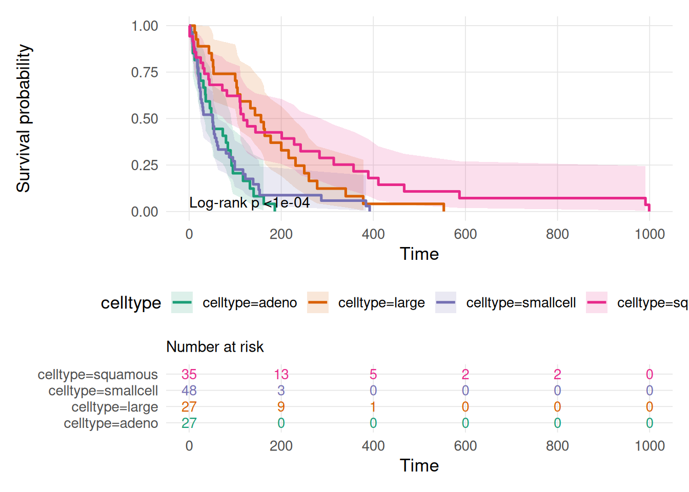
A consistent visual system: theme_survalis() and the color scales
Every plotting function used to call theme_minimal() with its own base_size, and grouped plots fell back to ggplot2’s default hue palette except for plot_survcurve(). theme_survalis() and the colorblind-friendly scale_color_survalis() / scale_fill_survalis() (ColorBrewer “Dark2”-based, interpolated beyond 8 levels) were retrofitted across every plotting function, plot_ale(), plot_pdp(), plot_shap(), plot_interactions(), plot_calibration(), plot_counterfactual(), plot_surrogate(), plot_tree_surrogate(), plot_varimp(), plot_survmat(), plot_survmetalearner_weights(), plot_benchmark(), cv_plot(), plot_survcurve(), so package figures read as one system instead of thirteen independent styles. Single-series hardcoded colors ("steelblue", "pink", "tomato", ad-hoc green/red hex codes) were replaced the same way, and every plot that can show both positive and negative values now draws a dashed zero-reference line.
As of 0.9.0, every one of those functions also takes a title argument: pass a custom string, leave it out for the previous auto-generated title, or pass title = NULL to drop it entirely for journals that require caption-only figures.
Uncertainty in variable importance: plot_varimp()
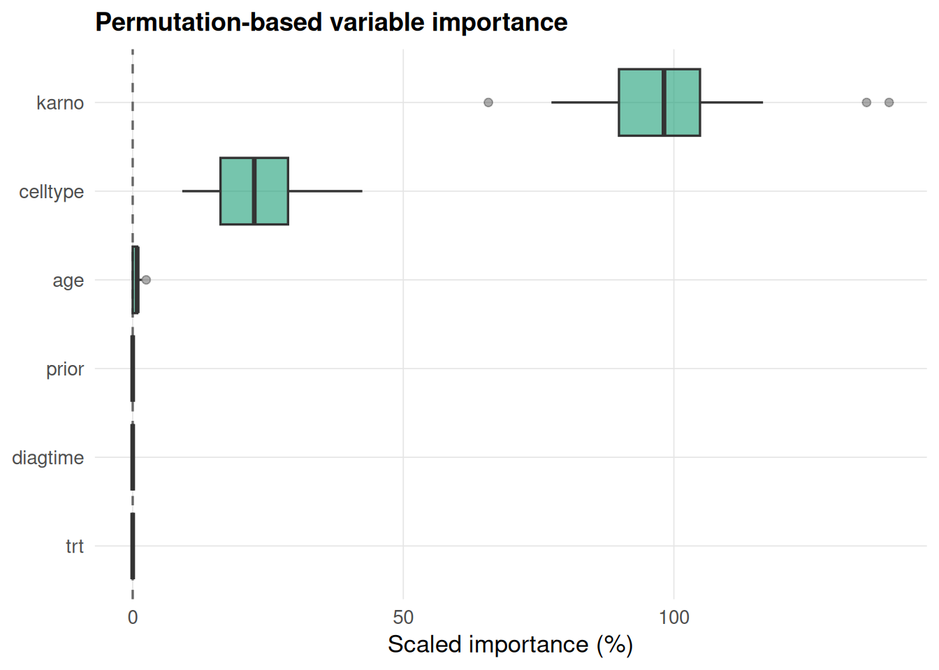
compute_varimp() computes permutation-based importance by repeating a metric drop over n_repetitions permutations per feature. It used to summarize those repetitions down to a single point estimate and discard them. plot_varimp() now draws the full per-repetition distribution as a boxplot instead of a lone point, and compute_varimp() keeps the raw values as a "raw_scores" attribute so the plot can use them (falling back to the old point-plot for hand-built summary tables without that attribute):
Migration to data.table
Every internal data-manipulation path, the CV/metrics engine (cv_survlearner(), cv_summary(), score_survmodel()), all nineteen tune_*() functions, cv_survmetalearner(), benchmark_tuned_survlearners(), compute_shap(), compute_calibration(), plot_survmat(), compute_varimp(), and the descriptive list_*() helpers, was migrated file by file from dplyr/tidyr/purrr/tibble to data.table. dplyr, tidyr, purrr, and tibble are no longer in Imports at all; data.table is now the sole data-manipulation engine. cv_summary()/score_survmodel() and summarise_benchmark() now round summary statistics to 3 decimals by default, consistently.
Corrections along the way
A few of these were silent correctness bugs, not just style:
-
auc_survmat()case definition. Cases were defined as events withtime <= t_starinstead of the canonical Uno/timeROCtime < t_star. This fed directly into the"auc"metric used throughoutscore_survmodel(),benchmark_*(), andfit_survmetalearner(), so it was corrected everywhere at once. -
Silently dropped learners in nested tuning.
benchmark_tuned_survlearners()selected tuning-result columns withtuning_results[1, cols, drop = FALSE], relying on data.frame[semantics; data.table’s[doesn’t select columns from a variable the same way, so every fold for a data.table-migrated learner errored and the learner was quietly dropped with a warning. Fixed with a.select_cols()helper that works for both data.frame/tibble and data.table inputs. -
tune_survsvm(refit_best = TRUE)crashes. A top-ranked grid candidate could fail to refit on the full dataset (aquadprogQP infeasibility that only shows up on certain BLAS backends, including CRAN’s OpenBLAS check machine). It now falls back to the next-best candidate and only errors if every candidate fails. -
plot_interactions(type = "heatmap")readability. Thewhite -> steelbluegradient had too little contrast in the mid-range and the zero-valued diagonal blended into the low end. Switched to a perceptually uniform viridis scale, flipped afterward so high interaction values read as dark rather than bright, matching conventional heatmap reading. -
plot_pdp()per-time facets. Free y-axis scales made survival-probability panels visually incomparable across facets; now fixed to[0, 1]viacoord_cartesian(). -
Stale generated docs breaking CI. Three
.Rdfiles had hand-drifted out of sync with their roxygen source, using\donttest{}(which CI runs) instead of\dontrun{}, causing an example to fail on an undefined object. Regenerated from source and verified withR CMD check --run-donttest.