unsurv: Unsupervised Clustering of Individualized Survival Curves

Survival analysis typically ends at the population level: a single estimated curve, or a hazard ratio summarizing the average effect of a covariate. But individualized survival curves, one per patient, open a richer question: can we identify subgroups of patients with similar prognosis trajectories, without ever labeling anyone in advance?

unsurv answers that question. It clusters individualized survival curves using Partitioning Around Medoids (PAM), with principled preprocessing choices (monotonic enforcement, weighted distances, automatic K selection) and a clean set of plotting helpers.

What is unsurv?

unsurv (v0.6.0) takes a matrix of survival probabilities (rows are subjects, columns are time points) and returns cluster assignments, medoid curves, and a silhouette diagnostic.

Install:

install.packages("unsurv")

The core idea

Suppose you have estimated individual survival curves \(S_i(t_1), \ldots, S_i(t_m)\) for \(n\) patients on a shared time grid \(t_1 < \cdots < t_m\) (from any model: Kaplan–Meier stratified by covariates, a Cox model, a random survival forest, or survdnn). Stack them into an \(n \times m\) matrix \(\mathbf{S}\) and pass it to unsurv().

The algorithm:

1. Optionally enforce monotone non-increasing curves.
2. Optionally smooth curves with a median filter.
3. Compute a weighted distance matrix (\(L_1\) or \(L_2\)) using trapezoidal weights by default, so time points in regions of faster change contribute more.
4. Run PAM on the distance matrix.
5. If \(K\) is unspecified, select the \(K \in \{2, \ldots, K_\text{max}\}\) that maximizes mean silhouette width.

Basic usage

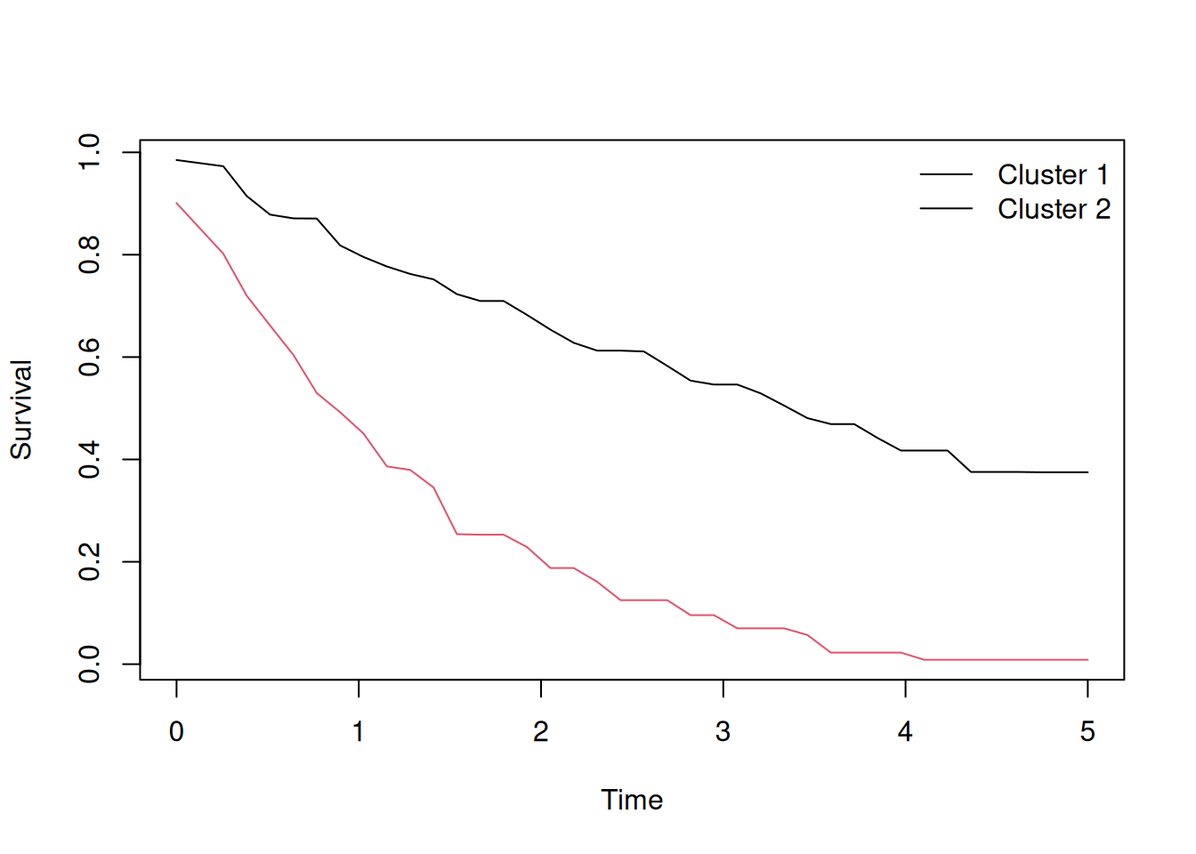
library(unsurv)

# Simulate survival curves from two latent risk groups
set.seed(42)
n     <- 100
times <- seq(0, 5, length.out = 40)
grp   <- sample(1:2, n, replace = TRUE)
rates <- ifelse(grp == 1, 0.2, 0.8)
S     <- outer(rates, times, function(r, t) exp(-r * t))
S     <- S + matrix(rnorm(n * length(times), sd = 0.02), nrow = n)

# Cluster with automatic K selection
fit <- unsurv(S, times, K = NULL, K_max = 6, seed = 123)

fit$K               # selected number of clusters

[1] 2

table(fit$clusters) # cluster assignment per subject

 1  2 
44 56 

fit$silhouette_mean # mean silhouette width at the selected K

[1] 0.9393843

Distance and weighting options

# L1 (Manhattan) distance: more robust to outlier curves
fit_l1 <- unsurv(S, times, K = 2, distance = "L1")

# Custom time weights: emphasize early time points
w <- rev(seq_along(times))
fit_w <- unsurv(S, times, K = 2, weights = w / sum(w))

Monotonic enforcement and smoothing

Raw predicted survival curves from flexible models may not be strictly non-increasing. unsurv corrects this before clustering:

fit <- unsurv(
  S, times, K = NULL, K_max = 6, seed = 123,
  enforce_monotone   = TRUE,  # project each curve to isotonic
  smooth_median_width = 5      # median filter of width 5 over time
)

Predicting clusters for new subjects

# newdata: n_new x m matrix of survival curves for new patients
pred <- predict(fit, newdata = S[1:5, ])
pred

[1] 1 1 1 1 2

Plotting

plot(fit)

Combining with a survival model

A natural pipeline is:

1. Fit individualized survival curves with a model of your choice (e.g., survdnn, rfsrc, Cox with spline terms).
2. Predict \(\hat{S}_i(t)\) on a common time grid.
3. Pass the resulting matrix to unsurv() to discover prognostic subgroups.
4. Use cluster membership as a stratification variable or as a phenotype to interrogate.

library(survival)
library(survdnn)
torch::torch_manual_seed(1)

dnn_fit <- survdnn(Surv(time, status) ~ age + sex + ph.ecog + ph.karno, data = lung,
                   hidden = c(64, 32), loss = "cox", epochs = 100, verbose = FALSE)

times_grid <- seq(0, 1000, by = 25)
S_hat <- as.matrix(predict(dnn_fit, newdata = lung, type = "survival", times = times_grid))

clust <- unsurv(S_hat, times_grid, K = NULL, K_max = 5, seed = 1)
table(clust$clusters)

  1   2   3 
113  70  43 

Methodological background

unsurv’s preprocessing choices, distance weighting, medoid-based clustering, and stability assessment are described in El Badisy (2026), “unsurv: Clustering Individualized Survival Curves”, Bioinformatics Advances, doi:10.1093/bioadv/vbag218, with a demonstration on the METABRIC breast cancer cohort using survdnn-predicted curves.

Links

• GitHub: github.com/ielbadisy/unsurv
• Paper: doi:10.1093/bioadv/vbag218