survdnn: Deep Neural Networks for Survival Analysis in R

Cox, AFT, and CoxTime losses with a formula interface, cross-validation, and calibration, powered by torch

survival-analysis

deep-learning

packages

Author

Imad El Badisy

Published

October 1, 2025

Survival analysis has traditionally been dominated by the Cox proportional hazards model and its semi-parametric extensions. Deep learning offers an alternative: one that can capture non-linear covariate effects and complex interactions without manual feature engineering. survdnn brings that capability to R via the torch backend, with the same formula-based interface that R users already know.

What is survdnn?

survdnn (v0.7.6) trains multilayer perceptrons for right-censored survival data. It supports four loss functions, built-in cross-validation, hyperparameter tuning, survival curve prediction, and standard evaluation metrics.

Install:

install.packages("torch")   # backend
install.packages("survdnn")

Fitting a model

The entry point is survdnn(), which takes a Surv() formula:

library(survival)
library(survdnn)
torch::torch_manual_seed(1)

fit <- survdnn(
  formula   = Surv(time, status) ~ age + sex + ph.ecog + ph.karno,
  data      = lung,
  hidden    = c(64, 32),
  activation = "relu",
  loss      = "cox",
  epochs    = 300,
  lr        = 1e-3,
  dropout   = 0.3,
  batch_norm = TRUE,
  verbose   = FALSE
)

fit

Loss functions

Four loss functions are available, covering the major families of deep survival models:

Loss	Model family	When to use
`"cox"`	Breslow Cox partial likelihood	Standard proportional hazards assumption
`"cox_l2"`	L2-penalized Cox	Regularization for wide feature sets
`"aft"`	Accelerated failure time	Log-linear relationship preferred
`"coxtime"`	CoxTime (Kvamme et al., JMLR 2019)	Time-varying covariate effects

Prediction and survival curves

# predict linear predictor (risk score)
head(predict(fit, newdata = lung, type = "lp"))

[1]  0.1397203 -0.2062566 -0.9678885  0.1454131 -0.7345585 -1.1179752

# predict survival curves on a time grid
times <- seq(0, 1000, by = 50)
surv  <- predict(fit, newdata = lung, type = "survival", times = times)
head(surv)

        t=0      t=50     t=100     t=150     t=200     t=250     t=300
1 0.9951746 0.9361534 0.8451717 0.7604267 0.6144562 0.5117045 0.4266991
2 0.9965835 0.9543929 0.8877925 0.8238434 0.7085186 0.6224762 0.5473946
3 0.9984034 0.9784408 0.9459462 0.9134979 0.8513897 0.8014476 0.7547645
4 0.9951471 0.9358008 0.8443605 0.7592386 0.6127502 0.5097510 0.4246295
5 0.9979842 0.9728526 0.9322323 0.8920343 0.8161431 0.7561600 0.7009718
6 0.9986257 0.9814173 0.9533005 0.9250892 0.8706953 0.8265549 0.7849473
      t=350     t=400     t=450     t=500     t=550      t=600      t=650
1 0.3291391 0.2446004 0.1935003 0.1582133 0.1135787 0.08159666 0.05483936
2 0.4555458 0.3692460 0.3128289 0.2712947 0.2145830 0.16981532 0.12819513
3 0.6927352 0.6280267 0.5812417 0.5438405 0.4874379 0.43699172 0.38323199
4 0.3270575 0.2426419 0.1916944 0.1565566 0.1121769 0.08043761 0.05393788
5 0.6290261 0.5557598 0.5039996 0.4633978 0.4035571 0.35155256 0.29784911
6 0.7290997 0.6700901 0.6268990 0.5920222 0.5387818 0.49043253 0.43803954
       t=700      t=750       t=800       t=850       t=900       t=950
1 0.03171439 0.01237621 0.007940308 0.004207006 0.001865832 0.001865832
2 0.08701532 0.04471476 0.032664382 0.020839752 0.011723673 0.011723673
3 0.31981080 0.23436366 0.202402368 0.164090863 0.125440661 0.125440661
4 0.03109568 0.01206975 0.007724095 0.004077636 0.001800081 0.001800081
5 0.23701727 0.16006584 0.133011865 0.102049314 0.072695858 0.072695858
6 0.37488195 0.28688417 0.252875078 0.211093807 0.167527461 0.167527461
       t=1000
1 0.001865832
2 0.011723673
3 0.125440661
4 0.001800081
5 0.072695858
6 0.167527461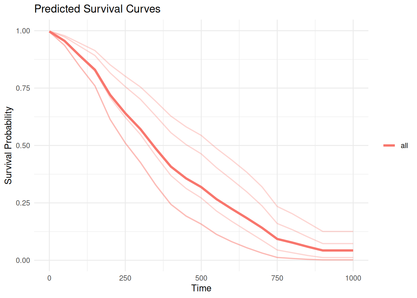

p <- plot(fit, newdata = lung[1:5, ], times = times)
ggplot2::ggsave("featured.png", p, width = 7, height = 4.5, dpi = 150)
p

Evaluation

evaluate_survdnn() computes the concordance index and integrated Brier score from the fitted model:

evaluate_survdnn(fit, metrics = c("cindex", "ibs"), times = seq(100, 800, by = 200), newdata = lung)

# A tibble: 2 × 2
  metric value
  <chr>  <dbl>
1 cindex 0.689
2 ibs    0.162

Hyperparameter tuning with cross-validation

tune_survdnn() runs a grid search over the hyperparameter space with K-fold cross-validation. param_grid is a named list crossed via tidyr::crossing(), and must include hidden, lr, activation, epochs, .loss_fn, and loss_name:

grid <- list(
  hidden     = list(c(16), c(32, 16)),
  lr         = c(1e-3, 1e-4),
  activation = c("relu"),
  epochs     = c(200),
  .loss_fn   = list(cox_loss, aft_loss),
  loss_name  = c("cox", "aft")
)

tuned <- tune_survdnn(
  formula = Surv(time, status) ~ age + sex + ph.ecog,
  data    = lung,
  times   = c(90, 300),
  metrics = "cindex",
  param_grid = grid,
  folds   = 5,
  return  = "summary"
)

Architecture

Under the hood, survdnn() builds an MLP via build_dnn(): linear layers with optional batch normalization and dropout between each hidden layer, terminating in a single linear output. The torch optimizer (Adam by default) is configurable via optimizer and optim_args.

Methodological background

survdnn’s design, loss functions, and benchmarks against classical and machine learning survival models are described in El Badisy (2026), “SurvDNN: Survival Deep Learning Models for Tabular Data”, The R Journal, RJ-2026-008.