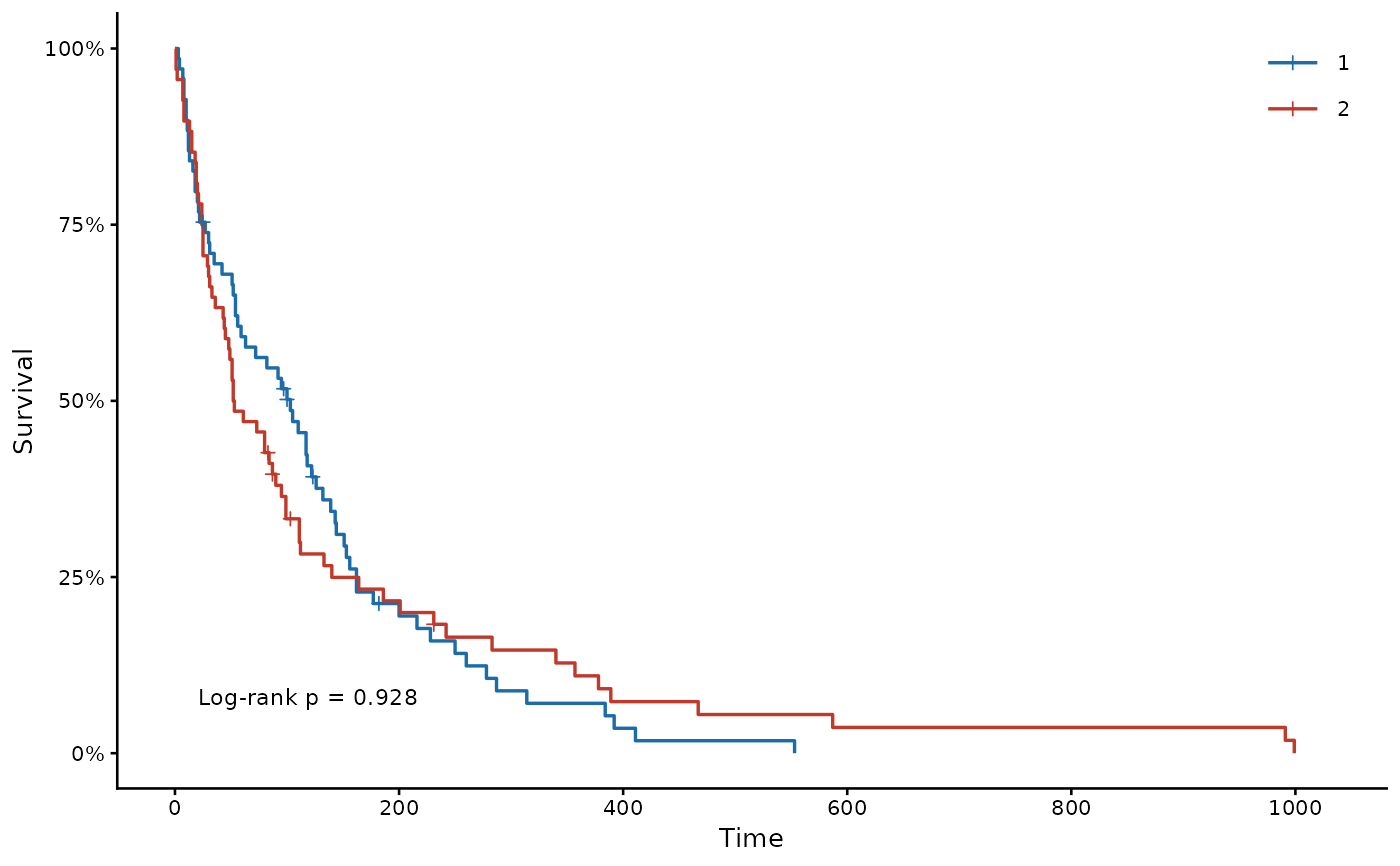
Kaplan-Meier curves with a number-at-risk table

Draws Kaplan-Meier curves in a publication style: step curves with censoring marks, the legend inside the panel, an optional log-rank p-value, and a number-at-risk table coloured by group under the plot. Besides the survival function, it draws the risk function, the cumulative hazard, the complementary log-log diagnostic of proportional hazards, and cumulative incidence under competing risks. A fitted survalis model adds its predicted or covariate-adjusted curves, dashed, over the Kaplan-Meier curves.

Usage

kmplot(
  formula,
  data,
  type = c("survival", "risk", "cumhaz", "cloglog"),
  event = NULL,
  model = NULL,
  model.curve = c("predicted", "adjusted"),
  title = NULL,
  xlab = "Time",
  ylab = NULL,
  breaks = NULL,
  pval = TRUE,
  risk.table = TRUE,
  conf.int = FALSE,
  colors = NULL,
  legend.pos = NULL,
  pval.pos = NULL,
  base_size = 10
)

Arguments

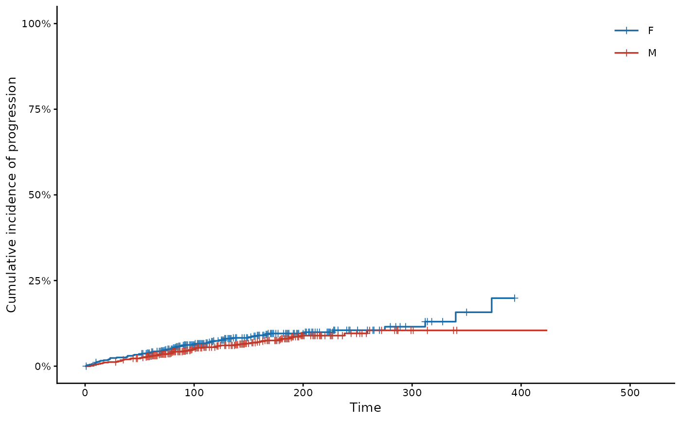
formula: A survival formula such as Surv(time, status) ~ 1 or Surv(time, status) ~ group, as in survival::survfit(). When the status is a factor whose first level is censoring and whose other levels are competing events, the plot shows the Aalen-Johansen cumulative incidence of event.
data: A data frame holding the variables in formula.
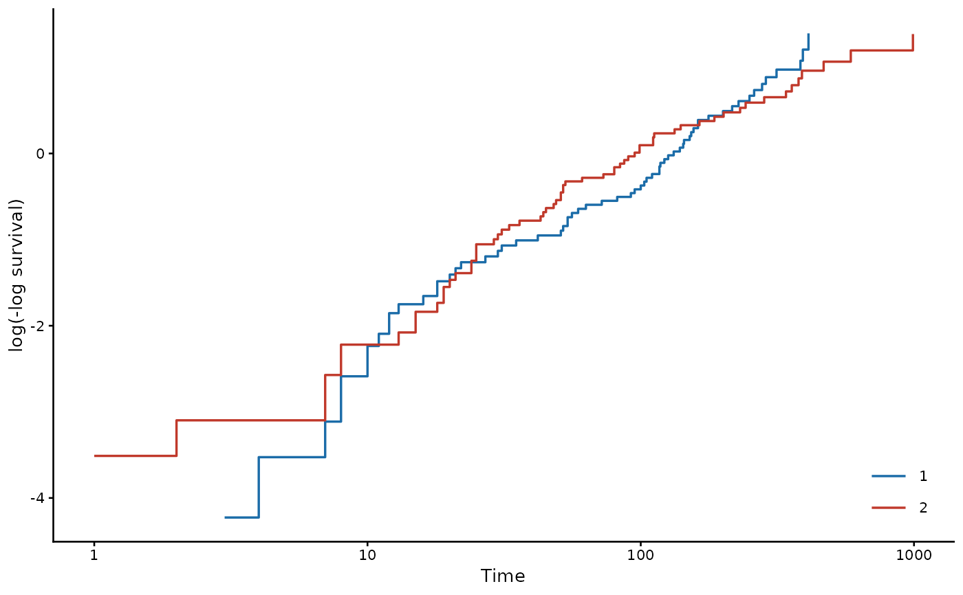
type: What to draw: "survival" (default) for \(S(t)\), "risk" for \(1 - S(t)\), "cumhaz" for the cumulative hazard \(H(t) = -\log S(t)\), or "cloglog" for \(\log\{-\log S(t)\}\) against \(\log t\), where parallel curves support proportional hazards. Competing-risks data take "risk" only, which is also their default.
event: Competing-risks data only: the event whose cumulative incidence is drawn. NULL (default) takes the first event level.
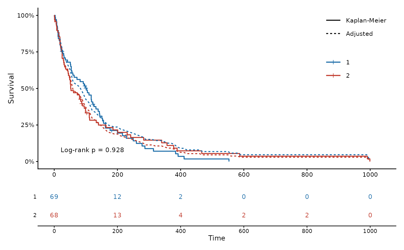
model: Optional fitted model from fit(). Its curves are drawn dashed over the Kaplan-Meier curves, so that the two can be compared. Not available for competing-risks data.
model.curve: "predicted" (default) averages the predicted survival of the subjects in each group, a calibration check of the model. "adjusted" sets the single grouping variable to each of its levels for every subject and averages the predictions (G-computation), which gives covariate-adjusted curves.
title: Panel title, for example "A. Overall survival". NULL (default) draws none.
xlab, ylab: Axis labels. ylab = NULL uses a label for type.
breaks: Time breaks for the x axis and the risk table. NULL (default) uses pretty() over the follow-up.
pval: Log-rank p-value when there are two or more groups: TRUE (default) computes it with survival::survdiff(), FALSE omits it, and a character string is printed as given. It is not computed for competing-risks data or for type = "cloglog", where only a string is printed.
risk.table: Logical; draw the number-at-risk table (default TRUE). Needs the 'patchwork' package. Not drawn for type = "cloglog", whose time axis is on the log scale.
conf.int: Logical; draw pointwise 95% confidence bands (default FALSE).
colors: Group colours. NULL (default) uses blue and red for the first two groups, then further distinct colours.
legend.pos: Legend position inside the panel, c(x, y) in [0, 1] units of the panel. NULL (default) chooses a corner away from the curves.
pval.pos: P-value position, c(time, y) in data units. NULL (default) chooses a corner away from the curves.
base_size: Base font size (default 10).

Value

A 'patchwork' object (curve over risk table) when the risk table is drawn, otherwise a 'ggplot2' object. Panels combine with patchwork operators, for example kmplot(...) | kmplot(...).

Examples

kmplot(Surv(time, status) ~ trt, data = veteran, risk.table = FALSE)

kmplot(Surv(time, status) ~ trt, data = veteran, type = "cloglog")


# Competing risks: progression versus death without progression
d <- survival::mgus2
d$etime <- ifelse(d$pstat == 1, d$ptime, d$futime)
d$event <- factor(ifelse(d$pstat == 1, 1, 2 * d$death), 0:2,
                  c("censored", "progression", "death"))
kmplot(Surv(etime, event) ~ sex, data = d, risk.table = FALSE)

# \donttest{
if (requireNamespace("patchwork", quietly = TRUE)) {
  kmplot(Surv(time, status) ~ trt, data = veteran,
         title = "A. Overall survival", xlab = "Days",
         breaks = seq(0, 1000, 200))

  # Covariate-adjusted curves from a Cox model, over the Kaplan-Meier curves
  m <- fit(Surv(time, status) ~ trt + karno + age, data = veteran,
           model = "coxph")
  kmplot(Surv(time, status) ~ trt, data = veteran, model = m,
         model.curve = "adjusted", breaks = seq(0, 1000, 200))
}

# }