Interpret a fitted survival learner

A single entry point to the package's model-agnostic explanation and diagnostic methods. listmethods() lists the method ids with a one-line description of each.

Usage

interpret(fit, method, newdata = NULL, data = NULL, times = NULL, ...)

Arguments

fit

A survalis_fit (from fit()), a survalis_tune, or a legacy mlsurv_model.

method

One of "pdp", "ice", "ale", "shap", "shap_matrix", "varimp" / "permute", "interaction", "counterfactual", "surrogate", "tree_surrogate", "calibration", "roc", "dca", "survcluster".

newdata

Instances to explain (SHAP, ALE, counterfactual, surrogate, survcluster) or to assess (roc, dca; these need the outcome columns). Defaults to data, so roc and dca are apparent unless you pass held-out data.

data

Background data for the method. Defaults to the training data.

times

Evaluation grid; NULL picks one from the data quantiles. Methods that need a single time (calibration, roc, dca) take eval_time in ... or the sole times value.

...

Method-specific arguments, e.g. feature (pdp / ice / ale), target_time (counterfactual, surrogate), eval_time (calibration, roc, dca), thresholds (dca), K (survcluster). For "shap", the aggregation over time ("meanabs" or "integral") is passed as shap_method.

Value

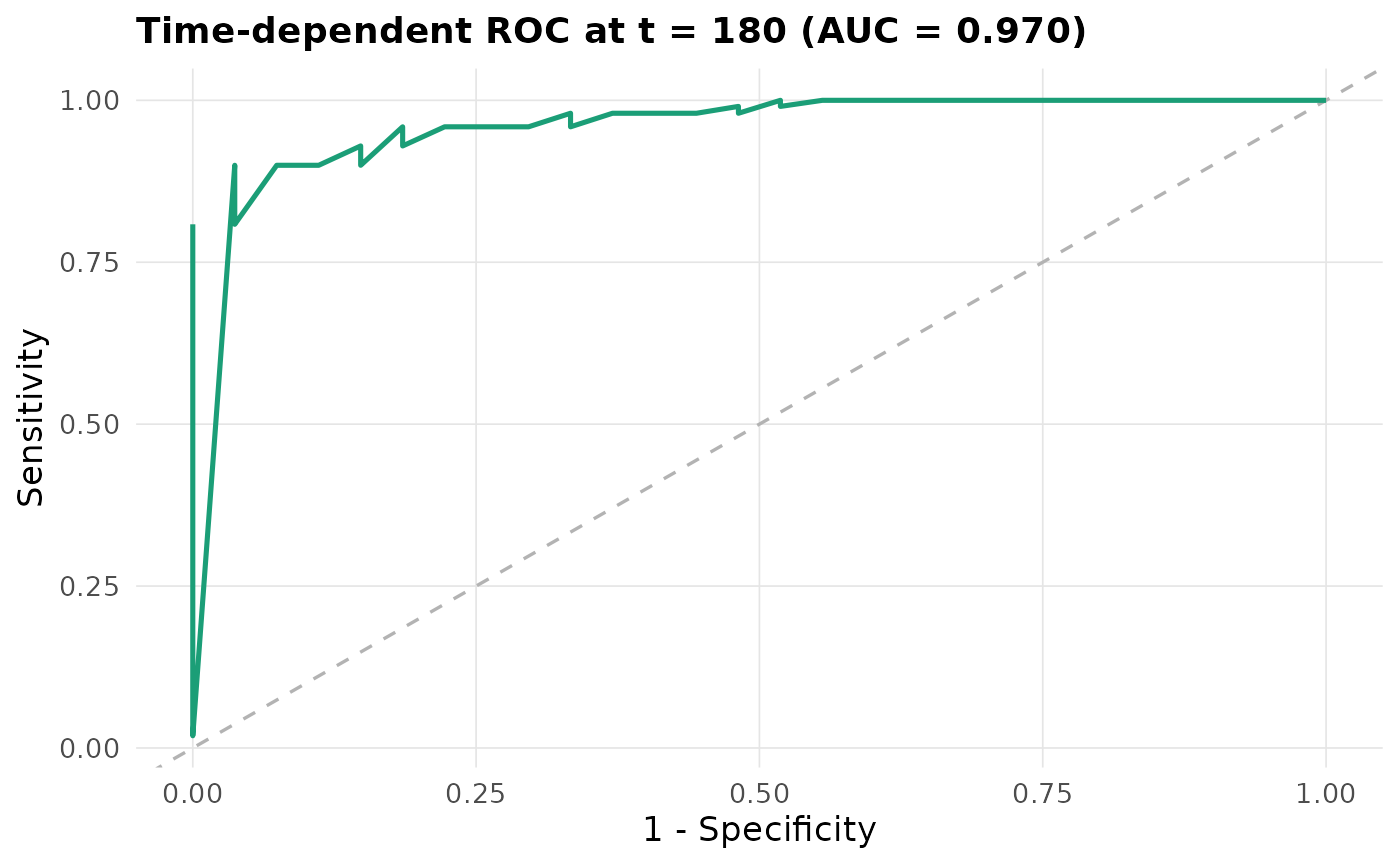
A survalis_interpret object holding the method's result, with method, times, and a plot() method. as.data.frame() returns the result frame. For "survcluster" it is in long format, one row per observation and time: id (row of newdata), cluster, medoid (TRUE for the cluster's medoid curve), time and predicted survival surv. For "roc" and "dca" it is the curve with an eval_time column (and auc for "roc"); for "tree_surrogate" one row per time and feature with the number of splits on it and the tree's r_squared. For "pdp" / "ice" it is one row per curve point (feature, feature_value, id (NA on PDP rows), time, surv, type), for "ale" one row per feature value and time (feature, feature_value, time, ale), and for "calibration" the binned table with its eval_time. For "pdp" and "ale", as.data.frame(x, what = "integrated") returns the curve integrated over time instead (feature, feature_value, integrated).

See also

For scalar summaries use evaluate(): metrics = "ece" summarises calibration and metrics = "auc" summarises the ROC curve.

Examples

m <- fit(Surv(time, status) ~ age + karno + celltype, veteran, "ranger",
         spec = list(num.trees = 100))
interpret(m, "pdp", feature = "karno", times = c(90, 180))
#> <survalis_interpret> method = pdp  |  model = ranger
#>   feature: karno 
#>   grid: 2 times in [90, 180]
#>   $result:
#>   feature feature_value id time      surv type
#> 1   karno      10.00000  1   90 0.2099627  ice
#> 2   karno      14.68421  1   90 0.2099627  ice
#> 3   karno      19.36842  1   90 0.2077350  ice
#> 4   karno      24.05263  1   90 0.2077350  ice
#> 5   karno      28.73684  1   90 0.2572695  ice
interpret(m, "varimp", times = c(90, 180))
#> <survalis_interpret> method = varimp  |  model = ranger
#>   grid: 2 times in [90, 180]
#>   $result:
#>    feature importance importance_05 importance_95 scaled_importance
#> 1    karno 0.13143405    0.10691343    0.16289422         100.00000
#> 2 celltype 0.07373054    0.05816584    0.08608992          56.09699
#> 3      age 0.03967214    0.02949784    0.04692894          30.18406
plot(interpret(m, "roc", eval_time = 180))